Channel Quality Assessment, Pruning, and Motion Artifact Detection

This notebook sketches how to prune bad channels and detect motion artefacts in fNIRS data

import cedalion
import cedalion.nirs
import cedalion.sigproc.quality as quality
import cedalion.xrutils as xrutils
import cedalion.datasets as datasets
import xarray as xr
import matplotlib.pyplot as p
from functools import reduce
import numpy as np

from cedalion import Quantity, units

# include matplotlib widget support in jupyter
# %matplotlib widget

Loading raw CW-NIRS data from a SNIRF file and converting it to OD and CONC

This notebook uses a finger-tapping dataset in BIDS layout provided by Rob Luke that is automatically fetched. You can also find it here.

# get example finger tapping dataset

snirf_element = datasets.get_fingertapping()
amp = snirf_element[0].data[0]
geo = snirf_element[0].geo3d
od = cedalion.nirs.int2od(amp)
# ml = snirf_element[0].measurement_lists[0]

data = xr.Dataset(
    data_vars = {
        "amp" : amp,
        "od"  : od,
        "geo3d": geo
    })


# Plot some data for visual validation
f,ax = p.subplots(1,1, figsize=(12,4))
ax.plot( data.amp.time, data.amp.sel(channel="S3D3", wavelength="850"), "r-", label="850nm")
ax.plot( data.amp.time, data.amp.sel(channel="S3D3", wavelength="760"), "r-", label="760nm")
p.legend()
ax.set_xlabel("time / s")
ax.set_ylabel("Signal intensity / a.u.")

amp.shape

(28, 2, 23239)

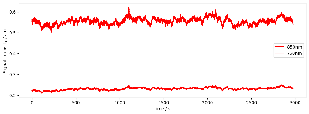
Calculating Signal Quality Metrics and applying Masks

To assess channel quality metrics such as SNR, channel distances, average amplitudes, sci, and others, we use small helper functions. As input, the quality functions should also expect thresholds for these metrics, so they can feed back both the calculated quality metrics as well as a mask. The masks can then be combined and applied - e.g. to prune channels with low SNR. The input and output arguments are based on xarray time series, quality parameters / instructions for thresholding. The returned mask is a boolean array in the shape and size of the input time series. It indicates where the threshold for our quality metric was passed (“True”) and is False otherwise. Mmsks can be combined with other masks, for instance to apply several metrics to assess or prune channels. At any point in time, the mask can be applied using the “apply_mask()” function available from cedalion’s the xrutils package.

If you are a user who is mainly interested in high-level application, you can skip to the Section “Channel Pruning using Quality Metrics and the Pruning Function” below. The “prune_ch()” function provides a higher abstraction layer to simply prune your data, using the same metrics and functions that are demonstrated below.

Channel Quality Metrics: SNR

# Here we assess channel quality by SNR
snr_thresh = 16 # the SNR (std/mean) of a channel. Set high here for demonstration purposes

# SNR thresholding using the "snr" function of the quality subpackage
snr, snr_mask = quality.snr(data.amp, snr_thresh)

# apply mask function. In this example, we want all signals with an SNR below the threshold to be replaced with "nan".
# We do not want to collapse / combine any dimension of the mask (last argument: "none")
data_masked_snr_1, masked_elements_1 = xrutils.apply_mask(data.amp, snr_mask, "nan", "none")

# alternatively, we can "drop" all channels with an SNR below the threshold. Since the SNR of both wavelength might differ
# (pass the threshold for one wavelength, but not for the other), we collapse to the "channel" dimension.
data_masked_snr_2, masked_elements_2 = xrutils.apply_mask(data.amp, snr_mask, "drop", "channel")

# show some results
print(f"channels that were masked according to the SNR threshold: {masked_elements_2}")

# dropped:
data_masked_snr_2

mask collapsed to channel dimension
channels that were masked according to the SNR threshold: ['S4D4' 'S5D7' 'S6D8' 'S8D8']

<xarray.DataArray 'amp' (channel: 24, wavelength: 2, time: 23239)> Size: 9MB
<Quantity([[[0.0913686 0.0909875 0.0910225 ... 0.0941083 0.0940129 0.0944882]
  [0.1856806 0.186377  0.1836514 ... 0.1856486 0.1850836 0.1842172]]

 [[0.227516  0.2297024 0.2261366 ... 0.2264519 0.2271665 0.226713 ]
  [0.6354927 0.637668  0.6298023 ... 0.6072068 0.6087293 0.6091066]]

 [[0.1064704 0.1066212 0.1053444 ... 0.121114  0.1205022 0.1205441]
  [0.2755033 0.2761615 0.2727006 ... 0.2911952 0.2900544 0.2909847]]

 ...

 [[0.187484  0.1868235 0.1866562 ... 0.1735965 0.1736705 0.1738339]
  [0.2424386 0.241503  0.2408491 ... 0.22303   0.2229887 0.2234081]]

 [[0.2027881 0.1996586 0.2004866 ... 0.2318743 0.2311941 0.2330808]
  [0.4666358 0.4554404 0.4561614 ... 0.4809749 0.4812827 0.4862896]]

 [[0.6304559 0.6284427 0.6287045 ... 0.6810626 0.6809573 0.6818709]
  [1.2285622 1.2205907 1.2190002 ... 1.2729124 1.2727222 1.2755645]]], 'volt')>
Coordinates:
  * time        (time) float64 186kB 0.0 0.128 0.256 ... 2.974e+03 2.974e+03
    samples     (time) int64 186kB 0 1 2 3 4 5 ... 23234 23235 23236 23237 23238
  * channel     (channel) object 192B 'S1D1' 'S1D2' 'S1D3' ... 'S8D7' 'S8D16'
    source      (channel) object 192B 'S1' 'S1' 'S1' 'S1' ... 'S7' 'S8' 'S8'
    detector    (channel) object 192B 'D1' 'D2' 'D3' 'D9' ... 'D15' 'D7' 'D16'
  * wavelength  (wavelength) float64 16B 760.0 850.0
Attributes:
    data_type_group:  unprocessed raw

xarray.DataArray

'amp'

• channel: 24
• wavelength: 2
• time: 23239

• [V] 0.09137 0.09099 0.09102 0.09044 ... 1.273 1.273 1.273 1.276

  Magnitude

  [[[0.0913686 0.0909875 0.0910225 ... 0.0941083 0.0940129 0.0944882] [0.1856806 0.186377 0.1836514 ... 0.1856486 0.1850836 0.1842172]] [[0.227516 0.2297024 0.2261366 ... 0.2264519 0.2271665 0.226713] [0.6354927 0.637668 0.6298023 ... 0.6072068 0.6087293 0.6091066]] [[0.1064704 0.1066212 0.1053444 ... 0.121114 0.1205022 0.1205441] [0.2755033 0.2761615 0.2727006 ... 0.2911952 0.2900544 0.2909847]] ... [[0.187484 0.1868235 0.1866562 ... 0.1735965 0.1736705 0.1738339] [0.2424386 0.241503 0.2408491 ... 0.22303 0.2229887 0.2234081]] [[0.2027881 0.1996586 0.2004866 ... 0.2318743 0.2311941 0.2330808] [0.4666358 0.4554404 0.4561614 ... 0.4809749 0.4812827 0.4862896]] [[0.6304559 0.6284427 0.6287045 ... 0.6810626 0.6809573 0.6818709] [1.2285622 1.2205907 1.2190002 ... 1.2729124 1.2727222 1.2755645]]]

  Units

  volt

• Coordinates: (6)
  • time
    (time)
    float64
    0.0 0.128 ... 2.974e+03 2.974e+03

    units :

    second

    array([0.000000e+00, 1.280000e-01, 2.560000e-01, ..., 2.974208e+03,
           2.974336e+03, 2.974464e+03])

  • samples
    (time)
    int64
    0 1 2 3 ... 23235 23236 23237 23238

    array([    0,     1,     2, ..., 23236, 23237, 23238])

  • channel
    (channel)
    object
    'S1D1' 'S1D2' ... 'S8D7' 'S8D16'

    array(['S1D1', 'S1D2', 'S1D3', 'S1D9', 'S2D1', 'S2D3', 'S2D4', 'S2D10', 'S3D2',
           'S3D3', 'S3D11', 'S4D3', 'S4D12', 'S5D5', 'S5D6', 'S5D13', 'S6D5',
           'S6D7', 'S6D14', 'S7D6', 'S7D7', 'S7D15', 'S8D7', 'S8D16'], dtype=object)

  • source
    (channel)
    object
    'S1' 'S1' 'S1' ... 'S7' 'S8' 'S8'

    array(['S1', 'S1', 'S1', 'S1', 'S2', 'S2', 'S2', 'S2', 'S3', 'S3', 'S3',
           'S4', 'S4', 'S5', 'S5', 'S5', 'S6', 'S6', 'S6', 'S7', 'S7', 'S7',
           'S8', 'S8'], dtype=object)

  • detector
    (channel)
    object
    'D1' 'D2' 'D3' ... 'D15' 'D7' 'D16'

    array(['D1', 'D2', 'D3', 'D9', 'D1', 'D3', 'D4', 'D10', 'D2', 'D3', 'D11',
           'D3', 'D12', 'D5', 'D6', 'D13', 'D5', 'D7', 'D14', 'D6', 'D7',
           'D15', 'D7', 'D16'], dtype=object)

  • wavelength
    (wavelength)
    float64
    760.0 850.0

    array([760., 850.])

• Indexes: (3)
  • time
    PandasIndex

    PandasIndex(Index([     0.0,    0.128,    0.256,    0.384,    0.512,     0.64,    0.768,
              0.896,    1.024,    1.152,
           ...
           2973.312,  2973.44, 2973.568, 2973.696, 2973.824, 2973.952,  2974.08,
           2974.208, 2974.336, 2974.464],
          dtype='float64', name='time', length=23239))

  • channel
    PandasIndex

    PandasIndex(Index(['S1D1', 'S1D2', 'S1D3', 'S1D9', 'S2D1', 'S2D3', 'S2D4', 'S2D10', 'S3D2',
           'S3D3', 'S3D11', 'S4D3', 'S4D12', 'S5D5', 'S5D6', 'S5D13', 'S6D5',
           'S6D7', 'S6D14', 'S7D6', 'S7D7', 'S7D15', 'S8D7', 'S8D16'],
          dtype='object', name='channel'))

  • wavelength
    PandasIndex

    PandasIndex(Index([760.0, 850.0], dtype='float64', name='wavelength'))

• Attributes: (1)

  data_type_group :

  unprocessed raw

Channel Quality Metrics: Channel Distance

# Here we assess channel distances. We might want to exclude very short or very long channels
sd_threshs = [1, 4.5]*units.cm # defines the lower and upper bounds for the source-detector separation that we would like to keep

# Source Detector Separation thresholding
ch_dist, sd_mask = quality.sd_dist(data.amp, data.geo3d, sd_threshs)
# print the channel distances
print(f"channel distances are: {ch_dist}")

# apply mask function. In this example, we want to "drop" all channels that do not fall inside sd_threshs
# i.e. drop channels shorter than 1cm and longer than 4.5cm. We want to collapse along the "channel" dimension.
data_masked_sd, masked_elements = xrutils.apply_mask(data.amp, sd_mask, "drop", "channel")

# display the resultings
print(f"channels that were masked according to the SD Distance thresholds: {masked_elements}")
data_masked_sd

channel distances are: <xarray.DataArray 'geo3d' (channel: 28)> Size: 224B
<Quantity([0.039 0.039 0.041 0.008 0.037 0.038 0.037 0.007 0.04  0.037 0.008 0.041
 0.034 0.008 0.039 0.039 0.041 0.008 0.037 0.037 0.037 0.008 0.04  0.037
 0.007 0.041 0.033 0.008], 'meter')>
Coordinates:
  * channel   (channel) object 224B 'S1D1' 'S1D2' 'S1D3' ... 'S8D8' 'S8D16'
    source    (channel) object 224B 'S1' 'S1' 'S1' 'S1' ... 'S7' 'S8' 'S8' 'S8'
    detector  (channel) object 224B 'D1' 'D2' 'D3' 'D9' ... 'D7' 'D8' 'D16'
mask collapsed to channel dimension
channels that were masked according to the SD Distance thresholds: ['S1D9' 'S2D10' 'S3D11' 'S4D12' 'S5D13' 'S6D14' 'S7D15' 'S8D16']

<xarray.DataArray 'amp' (channel: 20, wavelength: 2, time: 23239)> Size: 7MB
<Quantity([[[0.0913686 0.0909875 0.0910225 ... 0.0941083 0.0940129 0.0944882]
  [0.1856806 0.186377  0.1836514 ... 0.1856486 0.1850836 0.1842172]]

 [[0.227516  0.2297024 0.2261366 ... 0.2264519 0.2271665 0.226713 ]
  [0.6354927 0.637668  0.6298023 ... 0.6072068 0.6087293 0.6091066]]

 [[0.1064704 0.1066212 0.1053444 ... 0.121114  0.1205022 0.1205441]
  [0.2755033 0.2761615 0.2727006 ... 0.2911952 0.2900544 0.2909847]]

 ...

 [[0.2225884 0.2187791 0.2195495 ... 0.2564863 0.2551258 0.2560233]
  [0.3994258 0.3917637 0.389261  ... 0.4304597 0.430814  0.4331249]]

 [[0.2027881 0.1996586 0.2004866 ... 0.2318743 0.2311941 0.2330808]
  [0.4666358 0.4554404 0.4561614 ... 0.4809749 0.4812827 0.4862896]]

 [[0.4885007 0.4802285 0.4818338 ... 0.6109142 0.6108118 0.613845 ]
  [0.8457658 0.825988  0.8259648 ... 0.975894  0.9756599 0.9826459]]], 'volt')>
Coordinates:
  * time        (time) float64 186kB 0.0 0.128 0.256 ... 2.974e+03 2.974e+03
    samples     (time) int64 186kB 0 1 2 3 4 5 ... 23234 23235 23236 23237 23238
  * channel     (channel) object 160B 'S1D1' 'S1D2' 'S1D3' ... 'S8D7' 'S8D8'
    source      (channel) object 160B 'S1' 'S1' 'S1' 'S2' ... 'S7' 'S8' 'S8'
    detector    (channel) object 160B 'D1' 'D2' 'D3' 'D1' ... 'D7' 'D7' 'D8'
  * wavelength  (wavelength) float64 16B 760.0 850.0
Attributes:
    data_type_group:  unprocessed raw

xarray.DataArray

'amp'

• channel: 20
• wavelength: 2
• time: 23239

• [V] 0.09137 0.09099 0.09102 0.09044 ... 0.9732 0.9759 0.9757 0.9826

  Magnitude

  [[[0.0913686 0.0909875 0.0910225 ... 0.0941083 0.0940129 0.0944882] [0.1856806 0.186377 0.1836514 ... 0.1856486 0.1850836 0.1842172]] [[0.227516 0.2297024 0.2261366 ... 0.2264519 0.2271665 0.226713] [0.6354927 0.637668 0.6298023 ... 0.6072068 0.6087293 0.6091066]] [[0.1064704 0.1066212 0.1053444 ... 0.121114 0.1205022 0.1205441] [0.2755033 0.2761615 0.2727006 ... 0.2911952 0.2900544 0.2909847]] ... [[0.2225884 0.2187791 0.2195495 ... 0.2564863 0.2551258 0.2560233] [0.3994258 0.3917637 0.389261 ... 0.4304597 0.430814 0.4331249]] [[0.2027881 0.1996586 0.2004866 ... 0.2318743 0.2311941 0.2330808] [0.4666358 0.4554404 0.4561614 ... 0.4809749 0.4812827 0.4862896]] [[0.4885007 0.4802285 0.4818338 ... 0.6109142 0.6108118 0.613845] [0.8457658 0.825988 0.8259648 ... 0.975894 0.9756599 0.9826459]]]

  Units

  volt

• Coordinates: (6)
  • time
    (time)
    float64
    0.0 0.128 ... 2.974e+03 2.974e+03

    units :

    second

    array([0.000000e+00, 1.280000e-01, 2.560000e-01, ..., 2.974208e+03,
           2.974336e+03, 2.974464e+03])

  • samples
    (time)
    int64
    0 1 2 3 ... 23235 23236 23237 23238

    array([    0,     1,     2, ..., 23236, 23237, 23238])

  • channel
    (channel)
    object
    'S1D1' 'S1D2' ... 'S8D7' 'S8D8'

    array(['S1D1', 'S1D2', 'S1D3', 'S2D1', 'S2D3', 'S2D4', 'S3D2', 'S3D3', 'S4D3',
           'S4D4', 'S5D5', 'S5D6', 'S5D7', 'S6D5', 'S6D7', 'S6D8', 'S7D6', 'S7D7',
           'S8D7', 'S8D8'], dtype=object)

  • source
    (channel)
    object
    'S1' 'S1' 'S1' ... 'S7' 'S8' 'S8'

    array(['S1', 'S1', 'S1', 'S2', 'S2', 'S2', 'S3', 'S3', 'S4', 'S4', 'S5',
           'S5', 'S5', 'S6', 'S6', 'S6', 'S7', 'S7', 'S8', 'S8'], dtype=object)

  • detector
    (channel)
    object
    'D1' 'D2' 'D3' ... 'D7' 'D7' 'D8'

    array(['D1', 'D2', 'D3', 'D1', 'D3', 'D4', 'D2', 'D3', 'D3', 'D4', 'D5',
           'D6', 'D7', 'D5', 'D7', 'D8', 'D6', 'D7', 'D7', 'D8'], dtype=object)

  • wavelength
    (wavelength)
    float64
    760.0 850.0

    array([760., 850.])

• Indexes: (3)
  • time
    PandasIndex

    PandasIndex(Index([     0.0,    0.128,    0.256,    0.384,    0.512,     0.64,    0.768,
              0.896,    1.024,    1.152,
           ...
           2973.312,  2973.44, 2973.568, 2973.696, 2973.824, 2973.952,  2974.08,
           2974.208, 2974.336, 2974.464],
          dtype='float64', name='time', length=23239))

  • channel
    PandasIndex

    PandasIndex(Index(['S1D1', 'S1D2', 'S1D3', 'S2D1', 'S2D3', 'S2D4', 'S3D2', 'S3D3', 'S4D3',
           'S4D4', 'S5D5', 'S5D6', 'S5D7', 'S6D5', 'S6D7', 'S6D8', 'S7D6', 'S7D7',
           'S8D7', 'S8D8'],
          dtype='object', name='channel'))

  • wavelength
    PandasIndex

    PandasIndex(Index([760.0, 850.0], dtype='float64', name='wavelength'))

• Attributes: (1)

  data_type_group :

  unprocessed raw

Channel Quality Metrics: Mean Amplitudes

# Here we assess average channel amplitudes. We might want to exclude very small or large signals
amp_threshs = [0.1, 3]*units.volt # define whether a channel's amplitude is within a certain range

# Amplitude thresholding
mean_amp, amp_mask = quality.mean_amp(data.amp, amp_threshs)

# apply mask function. In this example, we want drop all channels that do not fall inside the amplitude thresholds.
# We collapse to the "channel" dimension.
data_masked_amp, masked_elements = xrutils.apply_mask(data.amp, amp_mask, "drop", "channel")

# display the results
print(f"channels that were masked according to the amplitude threshold: {masked_elements}")
data_masked_amp

mask collapsed to channel dimension
channels that were masked according to the amplitude threshold: ['S1D1' 'S1D9' 'S3D2' 'S6D8' 'S7D6']

<xarray.DataArray 'amp' (channel: 23, wavelength: 2, time: 23239)> Size: 9MB
<Quantity([[[0.227516  0.2297024 0.2261366 ... 0.2264519 0.2271665 0.226713 ]
  [0.6354927 0.637668  0.6298023 ... 0.6072068 0.6087293 0.6091066]]

 [[0.1064704 0.1066212 0.1053444 ... 0.121114  0.1205022 0.1205441]
  [0.2755033 0.2761615 0.2727006 ... 0.2911952 0.2900544 0.2909847]]

 [[0.5512474 0.5510672 0.5476283 ... 0.6179242 0.6188702 0.6187721]
  [1.125532  1.1238331 1.1119423 ... 1.1817728 1.1819598 1.1832658]]

 ...

 [[0.2027881 0.1996586 0.2004866 ... 0.2318743 0.2311941 0.2330808]
  [0.4666358 0.4554404 0.4561614 ... 0.4809749 0.4812827 0.4862896]]

 [[0.4885007 0.4802285 0.4818338 ... 0.6109142 0.6108118 0.613845 ]
  [0.8457658 0.825988  0.8259648 ... 0.975894  0.9756599 0.9826459]]

 [[0.6304559 0.6284427 0.6287045 ... 0.6810626 0.6809573 0.6818709]
  [1.2285622 1.2205907 1.2190002 ... 1.2729124 1.2727222 1.2755645]]], 'volt')>
Coordinates:
  * time        (time) float64 186kB 0.0 0.128 0.256 ... 2.974e+03 2.974e+03
    samples     (time) int64 186kB 0 1 2 3 4 5 ... 23234 23235 23236 23237 23238
  * channel     (channel) object 184B 'S1D2' 'S1D3' 'S2D1' ... 'S8D8' 'S8D16'
    source      (channel) object 184B 'S1' 'S1' 'S2' 'S2' ... 'S8' 'S8' 'S8'
    detector    (channel) object 184B 'D2' 'D3' 'D1' 'D3' ... 'D7' 'D8' 'D16'
  * wavelength  (wavelength) float64 16B 760.0 850.0
Attributes:
    data_type_group:  unprocessed raw

xarray.DataArray

'amp'

• channel: 23
• wavelength: 2
• time: 23239

• [V] 0.2275 0.2297 0.2261 0.2259 0.2267 ... 1.273 1.273 1.273 1.276

  Magnitude

  [[[0.227516 0.2297024 0.2261366 ... 0.2264519 0.2271665 0.226713] [0.6354927 0.637668 0.6298023 ... 0.6072068 0.6087293 0.6091066]] [[0.1064704 0.1066212 0.1053444 ... 0.121114 0.1205022 0.1205441] [0.2755033 0.2761615 0.2727006 ... 0.2911952 0.2900544 0.2909847]] [[0.5512474 0.5510672 0.5476283 ... 0.6179242 0.6188702 0.6187721] [1.125532 1.1238331 1.1119423 ... 1.1817728 1.1819598 1.1832658]] ... [[0.2027881 0.1996586 0.2004866 ... 0.2318743 0.2311941 0.2330808] [0.4666358 0.4554404 0.4561614 ... 0.4809749 0.4812827 0.4862896]] [[0.4885007 0.4802285 0.4818338 ... 0.6109142 0.6108118 0.613845] [0.8457658 0.825988 0.8259648 ... 0.975894 0.9756599 0.9826459]] [[0.6304559 0.6284427 0.6287045 ... 0.6810626 0.6809573 0.6818709] [1.2285622 1.2205907 1.2190002 ... 1.2729124 1.2727222 1.2755645]]]

  Units

  volt

• Coordinates: (6)
  • time
    (time)
    float64
    0.0 0.128 ... 2.974e+03 2.974e+03

    units :

    second

    array([0.000000e+00, 1.280000e-01, 2.560000e-01, ..., 2.974208e+03,
           2.974336e+03, 2.974464e+03])

  • samples
    (time)
    int64
    0 1 2 3 ... 23235 23236 23237 23238

    array([    0,     1,     2, ..., 23236, 23237, 23238])

  • channel
    (channel)
    object
    'S1D2' 'S1D3' ... 'S8D8' 'S8D16'

    array(['S1D2', 'S1D3', 'S2D1', 'S2D3', 'S2D4', 'S2D10', 'S3D3', 'S3D11',
           'S4D3', 'S4D4', 'S4D12', 'S5D5', 'S5D6', 'S5D7', 'S5D13', 'S6D5',
           'S6D7', 'S6D14', 'S7D7', 'S7D15', 'S8D7', 'S8D8', 'S8D16'], dtype=object)

  • source
    (channel)
    object
    'S1' 'S1' 'S2' ... 'S8' 'S8' 'S8'

    array(['S1', 'S1', 'S2', 'S2', 'S2', 'S2', 'S3', 'S3', 'S4', 'S4', 'S4',
           'S5', 'S5', 'S5', 'S5', 'S6', 'S6', 'S6', 'S7', 'S7', 'S8', 'S8',
           'S8'], dtype=object)

  • detector
    (channel)
    object
    'D2' 'D3' 'D1' ... 'D7' 'D8' 'D16'

    array(['D2', 'D3', 'D1', 'D3', 'D4', 'D10', 'D3', 'D11', 'D3', 'D4',
           'D12', 'D5', 'D6', 'D7', 'D13', 'D5', 'D7', 'D14', 'D7', 'D15',
           'D7', 'D8', 'D16'], dtype=object)

  • wavelength
    (wavelength)
    float64
    760.0 850.0

    array([760., 850.])

• Indexes: (3)
  • time
    PandasIndex

    PandasIndex(Index([     0.0,    0.128,    0.256,    0.384,    0.512,     0.64,    0.768,
              0.896,    1.024,    1.152,
           ...
           2973.312,  2973.44, 2973.568, 2973.696, 2973.824, 2973.952,  2974.08,
           2974.208, 2974.336, 2974.464],
          dtype='float64', name='time', length=23239))

  • channel
    PandasIndex

    PandasIndex(Index(['S1D2', 'S1D3', 'S2D1', 'S2D3', 'S2D4', 'S2D10', 'S3D3', 'S3D11',
           'S4D3', 'S4D4', 'S4D12', 'S5D5', 'S5D6', 'S5D7', 'S5D13', 'S6D5',
           'S6D7', 'S6D14', 'S7D7', 'S7D15', 'S8D7', 'S8D8', 'S8D16'],
          dtype='object', name='channel'))

  • wavelength
    PandasIndex

    PandasIndex(Index([760.0, 850.0], dtype='float64', name='wavelength'))

• Attributes: (1)

  data_type_group :

  unprocessed raw

Channel Pruning using Quality Metrics and the Pruning Function

To prune channels according to quality criteria, we do not have to manually go through the steps above. Instead, we can create quality masks for the metrics that we are interested in and hand them to a dedicated channel pruning function. The prune function expects a list of quality masks alongside a logical operator that defines how these masks should be combined.

# as above we use three metrics and define thresholds accordingly
snr_thresh = 16 # the SNR (std/mean) of a channel.
sd_threshs = [1, 4.5]*units.cm # defines the lower and upper bounds for the source-detector separation that we would like to keep
amp_threshs = [0.1, 3]*units.volt # define whether a channel's amplitude is within a certain range

# then we calculate the masks for each metric: SNR, SD distance and mean amplitude
_, snr_mask = quality.snr(data.amp, snr_thresh)
_, sd_mask = quality.sd_dist(data.amp, data.geo3d, sd_threshs)
_, amp_mask = quality.mean_amp(data.amp, amp_threshs)

# put all masks in a list
masks = [snr_mask, sd_mask, amp_mask]

# prune channels using the masks and the operator "all", which will keep only channels that pass all three metrics
amp_pruned, drop_list = quality.prune_ch(data.amp, masks, "all")

# print list of dropped channels
print(f"List of pruned channels: {drop_list}")
# display the new data xarray
amp_pruned

mask collapsed to channel dimension
List of pruned channels: ['S1D1' 'S1D9' 'S2D10' 'S3D2' 'S3D11' 'S4D4' 'S4D12' 'S5D7' 'S5D13' 'S6D8'
 'S6D14' 'S7D6' 'S7D15' 'S8D8' 'S8D16']

<xarray.DataArray 'amp' (channel: 13, wavelength: 2, time: 23239)> Size: 5MB
<Quantity([[[0.227516  0.2297024 0.2261366 ... 0.2264519 0.2271665 0.226713 ]
  [0.6354927 0.637668  0.6298023 ... 0.6072068 0.6087293 0.6091066]]

 [[0.1064704 0.1066212 0.1053444 ... 0.121114  0.1205022 0.1205441]
  [0.2755033 0.2761615 0.2727006 ... 0.2911952 0.2900544 0.2909847]]

 [[0.5512474 0.5510672 0.5476283 ... 0.6179242 0.6188702 0.6187721]
  [1.125532  1.1238331 1.1119423 ... 1.1817728 1.1819598 1.1832658]]

 ...

 [[0.3463254 0.3424951 0.3408207 ... 0.3929267 0.3941368 0.3945422]
  [0.6978315 0.6875081 0.6857653 ... 0.7259991 0.7271688 0.7292138]]

 [[0.2225884 0.2187791 0.2195495 ... 0.2564863 0.2551258 0.2560233]
  [0.3994258 0.3917637 0.389261  ... 0.4304597 0.430814  0.4331249]]

 [[0.2027881 0.1996586 0.2004866 ... 0.2318743 0.2311941 0.2330808]
  [0.4666358 0.4554404 0.4561614 ... 0.4809749 0.4812827 0.4862896]]], 'volt')>
Coordinates:
  * time        (time) float64 186kB 0.0 0.128 0.256 ... 2.974e+03 2.974e+03
    samples     (time) int64 186kB 0 1 2 3 4 5 ... 23234 23235 23236 23237 23238
  * channel     (channel) object 104B 'S1D2' 'S1D3' 'S2D1' ... 'S7D7' 'S8D7'
    source      (channel) object 104B 'S1' 'S1' 'S2' 'S2' ... 'S6' 'S7' 'S8'
    detector    (channel) object 104B 'D2' 'D3' 'D1' 'D3' ... 'D7' 'D7' 'D7'
  * wavelength  (wavelength) float64 16B 760.0 850.0
Attributes:
    data_type_group:  unprocessed raw

xarray.DataArray

'amp'

• channel: 13
• wavelength: 2
• time: 23239

• [V] 0.2275 0.2297 0.2261 0.2259 0.2267 ... 0.4808 0.481 0.4813 0.4863

  Magnitude

  [[[0.227516 0.2297024 0.2261366 ... 0.2264519 0.2271665 0.226713] [0.6354927 0.637668 0.6298023 ... 0.6072068 0.6087293 0.6091066]] [[0.1064704 0.1066212 0.1053444 ... 0.121114 0.1205022 0.1205441] [0.2755033 0.2761615 0.2727006 ... 0.2911952 0.2900544 0.2909847]] [[0.5512474 0.5510672 0.5476283 ... 0.6179242 0.6188702 0.6187721] [1.125532 1.1238331 1.1119423 ... 1.1817728 1.1819598 1.1832658]] ... [[0.3463254 0.3424951 0.3408207 ... 0.3929267 0.3941368 0.3945422] [0.6978315 0.6875081 0.6857653 ... 0.7259991 0.7271688 0.7292138]] [[0.2225884 0.2187791 0.2195495 ... 0.2564863 0.2551258 0.2560233] [0.3994258 0.3917637 0.389261 ... 0.4304597 0.430814 0.4331249]] [[0.2027881 0.1996586 0.2004866 ... 0.2318743 0.2311941 0.2330808] [0.4666358 0.4554404 0.4561614 ... 0.4809749 0.4812827 0.4862896]]]

  Units

  volt

• Coordinates: (6)
  • time
    (time)
    float64
    0.0 0.128 ... 2.974e+03 2.974e+03

    units :

    second

    array([0.000000e+00, 1.280000e-01, 2.560000e-01, ..., 2.974208e+03,
           2.974336e+03, 2.974464e+03])

  • samples
    (time)
    int64
    0 1 2 3 ... 23235 23236 23237 23238

    array([    0,     1,     2, ..., 23236, 23237, 23238])

  • channel
    (channel)
    object
    'S1D2' 'S1D3' ... 'S7D7' 'S8D7'

    array(['S1D2', 'S1D3', 'S2D1', 'S2D3', 'S2D4', 'S3D3', 'S4D3', 'S5D5', 'S5D6',
           'S6D5', 'S6D7', 'S7D7', 'S8D7'], dtype=object)

  • source
    (channel)
    object
    'S1' 'S1' 'S2' ... 'S6' 'S7' 'S8'

    array(['S1', 'S1', 'S2', 'S2', 'S2', 'S3', 'S4', 'S5', 'S5', 'S6', 'S6',
           'S7', 'S8'], dtype=object)

  • detector
    (channel)
    object
    'D2' 'D3' 'D1' ... 'D7' 'D7' 'D7'

    array(['D2', 'D3', 'D1', 'D3', 'D4', 'D3', 'D3', 'D5', 'D6', 'D5', 'D7',
           'D7', 'D7'], dtype=object)

  • wavelength
    (wavelength)
    float64
    760.0 850.0

    array([760., 850.])

• Indexes: (3)
  • time
    PandasIndex

    PandasIndex(Index([     0.0,    0.128,    0.256,    0.384,    0.512,     0.64,    0.768,
              0.896,    1.024,    1.152,
           ...
           2973.312,  2973.44, 2973.568, 2973.696, 2973.824, 2973.952,  2974.08,
           2974.208, 2974.336, 2974.464],
          dtype='float64', name='time', length=23239))

  • channel
    PandasIndex

    PandasIndex(Index(['S1D2', 'S1D3', 'S2D1', 'S2D3', 'S2D4', 'S3D3', 'S4D3', 'S5D5', 'S5D6',
           'S6D5', 'S6D7', 'S7D7', 'S8D7'],
          dtype='object', name='channel'))

  • wavelength
    PandasIndex

    PandasIndex(Index([760.0, 850.0], dtype='float64', name='wavelength'))

• Attributes: (1)

  data_type_group :

  unprocessed raw

Motion Artefact Detection

The same xarray-based masks can be used for indicating motion-artefacts. The example below shows how to checks channels for motion artefacts using standard thresholds from Homer2/3. The output is a mask that can be handed to motion correction algorithms

Detecting Motion Artifacts and generating the MA mask

import cedalion.sigproc.artifact as artifact
import pandas as pd

# we use Optical Density data for motion artifact detection
fNIRSdata = data.od

# define parameters for motion artifact detection. We follow the method from Homer2/3: "hmrR_MotionArtifactByChannel" and "hmrR_MotionArtifact".
t_motion = 0.5*units.s  # time window for motion artifact detection
t_mask = 1.0*units.s    # time window for masking motion artifacts (+- t_mask s before/after detected motion artifact)
stdev_thresh = 4.0      # threshold for standard deviation of the signal used to detect motion artifacts. Default is 50. We set it very low to find something in our good data for demonstration purposes.
amp_thresh = 5.0        # threshold for amplitude of the signal used to detect motion artifacts. Default is 5.

# to identify motion artifacts with these parameters we call the following function
ma_mask = artifact.id_motion(fNIRSdata, t_motion, t_mask, stdev_thresh, amp_thresh)
# it hands us a boolean mask (xarray) of the input dimension, where True a element indicates a motion artifact at a given time point.

# show the masks data
ma_mask

/home/runner/micromamba/envs/cedalion/lib/python3.11/site-packages/xarray/core/variable.py:338: UnitStrippedWarning: The unit of the quantity is stripped when downcasting to ndarray.
  data = np.asarray(data)
/home/runner/micromamba/envs/cedalion/lib/python3.11/site-packages/xarray/core/variable.py:338: UnitStrippedWarning: The unit of the quantity is stripped when downcasting to ndarray.
  data = np.asarray(data)

<xarray.DataArray 'od' (channel: 28, wavelength: 2, time: 23239)> Size: 1MB
array([[[False, False, False, ..., False, False, False],
        [False, False, False, ..., False, False, False]],

       [[False, False, False, ..., False, False, False],
        [False, False, False, ..., False, False, False]],

       [[False, False, False, ..., False, False, False],
        [False, False, False, ..., False, False, False]],

       ...,

       [[False, False, False, ..., False, False, False],
        [False, False, False, ..., False, False, False]],

       [[False, False, False, ..., False, False, False],
        [False, False, False, ..., False, False, False]],

       [[False, False, False, ..., False, False, False],
        [ True,  True,  True, ..., False, False, False]]])
Coordinates:
  * time        (time) float64 186kB 0.0 0.128 0.256 ... 2.974e+03 2.974e+03
    samples     (time) int64 186kB 0 1 2 3 4 5 ... 23234 23235 23236 23237 23238
  * channel     (channel) object 224B 'S1D1' 'S1D2' 'S1D3' ... 'S8D8' 'S8D16'
    source      (channel) object 224B 'S1' 'S1' 'S1' 'S1' ... 'S8' 'S8' 'S8'
    detector    (channel) object 224B 'D1' 'D2' 'D3' 'D9' ... 'D7' 'D8' 'D16'
  * wavelength  (wavelength) float64 16B 760.0 850.0

xarray.DataArray

'od'

• channel: 28
• wavelength: 2
• time: 23239

• False False False False False False ... False False False False False

  array([[[False, False, False, ..., False, False, False],
          [False, False, False, ..., False, False, False]],
  
         [[False, False, False, ..., False, False, False],
          [False, False, False, ..., False, False, False]],
  
         [[False, False, False, ..., False, False, False],
          [False, False, False, ..., False, False, False]],
  
         ...,
  
         [[False, False, False, ..., False, False, False],
          [False, False, False, ..., False, False, False]],
  
         [[False, False, False, ..., False, False, False],
          [False, False, False, ..., False, False, False]],
  
         [[False, False, False, ..., False, False, False],
          [ True,  True,  True, ..., False, False, False]]])

• Coordinates: (6)
  • time
    (time)
    float64
    0.0 0.128 ... 2.974e+03 2.974e+03

    units :

    second

    array([0.000000e+00, 1.280000e-01, 2.560000e-01, ..., 2.974208e+03,
           2.974336e+03, 2.974464e+03])

  • samples
    (time)
    int64
    0 1 2 3 ... 23235 23236 23237 23238

    array([    0,     1,     2, ..., 23236, 23237, 23238])

  • channel
    (channel)
    object
    'S1D1' 'S1D2' ... 'S8D8' 'S8D16'

    array(['S1D1', 'S1D2', 'S1D3', 'S1D9', 'S2D1', 'S2D3', 'S2D4', 'S2D10', 'S3D2',
           'S3D3', 'S3D11', 'S4D3', 'S4D4', 'S4D12', 'S5D5', 'S5D6', 'S5D7',
           'S5D13', 'S6D5', 'S6D7', 'S6D8', 'S6D14', 'S7D6', 'S7D7', 'S7D15',
           'S8D7', 'S8D8', 'S8D16'], dtype=object)

  • source
    (channel)
    object
    'S1' 'S1' 'S1' ... 'S8' 'S8' 'S8'

    array(['S1', 'S1', 'S1', 'S1', 'S2', 'S2', 'S2', 'S2', 'S3', 'S3', 'S3',
           'S4', 'S4', 'S4', 'S5', 'S5', 'S5', 'S5', 'S6', 'S6', 'S6', 'S6',
           'S7', 'S7', 'S7', 'S8', 'S8', 'S8'], dtype=object)

  • detector
    (channel)
    object
    'D1' 'D2' 'D3' ... 'D7' 'D8' 'D16'

    array(['D1', 'D2', 'D3', 'D9', 'D1', 'D3', 'D4', 'D10', 'D2', 'D3', 'D11',
           'D3', 'D4', 'D12', 'D5', 'D6', 'D7', 'D13', 'D5', 'D7', 'D8',
           'D14', 'D6', 'D7', 'D15', 'D7', 'D8', 'D16'], dtype=object)

  • wavelength
    (wavelength)
    float64
    760.0 850.0

    array([760., 850.])

• Indexes: (3)
  • time
    PandasIndex

    PandasIndex(Index([     0.0,    0.128,    0.256,    0.384,    0.512,     0.64,    0.768,
              0.896,    1.024,    1.152,
           ...
           2973.312,  2973.44, 2973.568, 2973.696, 2973.824, 2973.952,  2974.08,
           2974.208, 2974.336, 2974.464],
          dtype='float64', name='time', length=23239))

  • channel
    PandasIndex

    PandasIndex(Index(['S1D1', 'S1D2', 'S1D3', 'S1D9', 'S2D1', 'S2D3', 'S2D4', 'S2D10', 'S3D2',
           'S3D3', 'S3D11', 'S4D3', 'S4D4', 'S4D12', 'S5D5', 'S5D6', 'S5D7',
           'S5D13', 'S6D5', 'S6D7', 'S6D8', 'S6D14', 'S7D6', 'S7D7', 'S7D15',
           'S8D7', 'S8D8', 'S8D16'],
          dtype='object', name='channel'))

  • wavelength
    PandasIndex

    PandasIndex(Index([760.0, 850.0], dtype='float64', name='wavelength'))

• Attributes: (0)

The output mask is quite detailed and still contains all original dimensions (e.g. single wavelengths) and allows us to combine it with a mask from another motion artifact detection method. This is the same approach as for the channel quality metrics above. While in quality metrics a “True” in the mask meant that the sample was above the quality threshold (“good”), in motion artifact masks a “True” represents an artifact. To invert the logic, simply use the boolean “not” operator “~”: ma_mask_inverted = ~ma_mask.

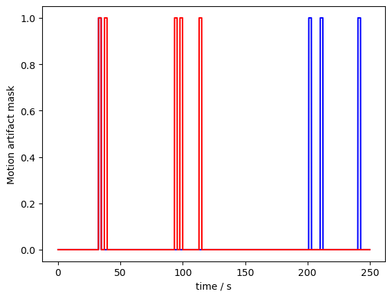
Let us now plot the result for an example channel. Note, that for both wavelengths a different number of artifacts was identified, which can sometimes happen:

p.figure()
p.plot(ma_mask.sel(time=slice(0,250)).time, ma_mask.sel(channel="S3D3", wavelength="760", time=slice(0,250)), "b-")
p.plot(ma_mask.sel(time=slice(0,250)).time, ma_mask.sel(channel="S3D3", wavelength="850", time=slice(0,250)), "r-")
p.xlabel("time / s")
p.ylabel("Motion artifact mask")
p.show()

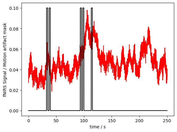
Our example dataset is very clean. So we artificially detected motion artifacts with a very low threshold. Plotting the mask and the data together (we have to rescale a bit to make both fit):

p.figure()
p.plot(fNIRSdata.sel(time=slice(0,250)).time, fNIRSdata.sel(channel="S3D3", wavelength="760", time=slice(0,250)), "r-")
p.plot(ma_mask.sel(time=slice(0,250)).time, ma_mask.sel(channel="S3D3", wavelength="850", time=slice(0,250))/10, "k-")
p.xlabel("time / s")
p.ylabel("fNIRS Signal / Motion artifact mask")
p.show()

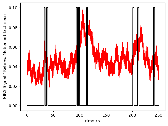
Refining the MA Mask

At the latest when we want to correct motion artifacts, we usually do not need the level of granularity that the mask provides. For instance, we usually want to treat a detected motion artifact in either of both wavelengths or chromophores of one channel as a single artifact that gets flagged for both. We might also want to flag motion artifacts globally, i.e. mask time points for all channels even if only some of them show an artifact. This can easily be done by using the “id_motion_refine” function. The function also returns useful information about motion artifacts in each channel in “ma_info”

# refine the motion artifact mask. This function collapses the mask along dimensions that are chosen by the "operator" argument.
# Here we use "by_channel", which will yield a mask for each channel by collapsing the masks along either the wavelength or concentration dimension.
ma_mask_refined, ma_info = artifact.id_motion_refine(ma_mask, 'by_channel')

# show the refined mask
ma_mask_refined

<xarray.DataArray 'od' (channel: 28, time: 23239)> Size: 651kB
array([[False, False, False, ..., False, False, False],
       [False, False, False, ..., False, False, False],
       [False, False, False, ..., False, False, False],
       ...,
       [False, False, False, ..., False, False, False],
       [False, False, False, ..., False, False, False],
       [ True,  True,  True, ..., False, False, False]])
Coordinates:
  * time      (time) float64 186kB 0.0 0.128 0.256 ... 2.974e+03 2.974e+03
    samples   (time) int64 186kB 0 1 2 3 4 5 ... 23234 23235 23236 23237 23238
  * channel   (channel) object 224B 'S1D1' 'S1D2' 'S1D3' ... 'S8D8' 'S8D16'
    source    (channel) object 224B 'S1' 'S1' 'S1' 'S1' ... 'S7' 'S8' 'S8' 'S8'
    detector  (channel) object 224B 'D1' 'D2' 'D3' 'D9' ... 'D7' 'D8' 'D16'

xarray.DataArray

'od'

• channel: 28
• time: 23239

• False False False False False True ... False False False False False

  array([[False, False, False, ..., False, False, False],
         [False, False, False, ..., False, False, False],
         [False, False, False, ..., False, False, False],
         ...,
         [False, False, False, ..., False, False, False],
         [False, False, False, ..., False, False, False],
         [ True,  True,  True, ..., False, False, False]])

• Coordinates: (5)
  • time
    (time)
    float64
    0.0 0.128 ... 2.974e+03 2.974e+03

    units :

    second

    array([0.000000e+00, 1.280000e-01, 2.560000e-01, ..., 2.974208e+03,
           2.974336e+03, 2.974464e+03])

  • samples
    (time)
    int64
    0 1 2 3 ... 23235 23236 23237 23238

    array([    0,     1,     2, ..., 23236, 23237, 23238])

  • channel
    (channel)
    object
    'S1D1' 'S1D2' ... 'S8D8' 'S8D16'

    array(['S1D1', 'S1D2', 'S1D3', 'S1D9', 'S2D1', 'S2D3', 'S2D4', 'S2D10', 'S3D2',
           'S3D3', 'S3D11', 'S4D3', 'S4D4', 'S4D12', 'S5D5', 'S5D6', 'S5D7',
           'S5D13', 'S6D5', 'S6D7', 'S6D8', 'S6D14', 'S7D6', 'S7D7', 'S7D15',
           'S8D7', 'S8D8', 'S8D16'], dtype=object)

  • source
    (channel)
    object
    'S1' 'S1' 'S1' ... 'S8' 'S8' 'S8'

    array(['S1', 'S1', 'S1', 'S1', 'S2', 'S2', 'S2', 'S2', 'S3', 'S3', 'S3',
           'S4', 'S4', 'S4', 'S5', 'S5', 'S5', 'S5', 'S6', 'S6', 'S6', 'S6',
           'S7', 'S7', 'S7', 'S8', 'S8', 'S8'], dtype=object)

  • detector
    (channel)
    object
    'D1' 'D2' 'D3' ... 'D7' 'D8' 'D16'

    array(['D1', 'D2', 'D3', 'D9', 'D1', 'D3', 'D4', 'D10', 'D2', 'D3', 'D11',
           'D3', 'D4', 'D12', 'D5', 'D6', 'D7', 'D13', 'D5', 'D7', 'D8',
           'D14', 'D6', 'D7', 'D15', 'D7', 'D8', 'D16'], dtype=object)

• Indexes: (2)
  • time
    PandasIndex

    PandasIndex(Index([     0.0,    0.128,    0.256,    0.384,    0.512,     0.64,    0.768,
              0.896,    1.024,    1.152,
           ...
           2973.312,  2973.44, 2973.568, 2973.696, 2973.824, 2973.952,  2974.08,
           2974.208, 2974.336, 2974.464],
          dtype='float64', name='time', length=23239))

  • channel
    PandasIndex

    PandasIndex(Index(['S1D1', 'S1D2', 'S1D3', 'S1D9', 'S2D1', 'S2D3', 'S2D4', 'S2D10', 'S3D2',
           'S3D3', 'S3D11', 'S4D3', 'S4D4', 'S4D12', 'S5D5', 'S5D6', 'S5D7',
           'S5D13', 'S6D5', 'S6D7', 'S6D8', 'S6D14', 'S7D6', 'S7D7', 'S7D15',
           'S8D7', 'S8D8', 'S8D16'],
          dtype='object', name='channel'))

• Attributes: (0)

Now the mask does not have the “wavelength” or “concentration” dimension anymore, and the masks of these dimensions are combined:

# plot the figure

p.figure()
p.plot(fNIRSdata.sel(time=slice(0,250)).time, fNIRSdata.sel(channel="S3D3", wavelength="760", time=slice(0,250)), "r-")
p.plot(ma_mask_refined.sel(time=slice(0,250)).time, ma_mask_refined.sel(channel="S3D3", time=slice(0,250))/10, "k-")
p.xlabel("time / s")
p.ylabel("fNIRS Signal / Refined Motion artifact mask")
p.show()

# show the information about the motion artifacts: we get a pandas dataframe telling us
# 1) for which channels artifacts were detected,
# 2) what is the fraction of time points that were marked as artifacts and
# 3) how many artifacts where detected
ma_info

	channel	ma_fraction	ma_count
0	S1D1	0.097379	105
1	S1D2	0.055854	64
2	S1D3	0.040105	48
3	S1D9	0.070141	89
4	S2D1	0.022161	28
5	S2D3	0.041439	47
6	S2D4	0.026894	20
7	S2D10	0.091484	100
8	S3D2	0.013254	18
9	S3D3	0.035888	46
10	S3D11	0.095142	101
11	S4D3	0.023925	25
12	S4D4	0.042300	29
13	S4D12	0.066440	58
14	S5D5	0.081372	93
15	S5D6	0.048023	57
16	S5D7	0.044064	54
17	S5D13	0.135075	126
18	S6D5	0.031628	34
19	S6D7	0.037652	46
20	S6D8	0.037738	34
21	S6D14	0.086751	87
22	S7D6	0.062266	71
23	S7D7	0.048152	52
24	S7D15	0.122079	126
25	S8D7	0.028831	34
26	S8D8	0.030767	19
27	S8D16	0.055037	52

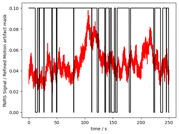
Now we look at the “all” operator, which will collapse the mask across all dimensions except time, leading to a single motion artifact mask

# "all", yields a mask that flags an artifact at any given time if flagged for any channel, wavelength, chromophore, etc.
ma_mask_refined, ma_info = artifact.id_motion_refine(ma_mask, 'all')

# show the refined mask
ma_mask_refined

<xarray.DataArray 'od' (time: 23239)> Size: 23kB
array([ True,  True,  True, ..., False, False, False])
Coordinates:
  * time     (time) float64 186kB 0.0 0.128 0.256 ... 2.974e+03 2.974e+03
    samples  (time) int64 186kB 0 1 2 3 4 5 ... 23234 23235 23236 23237 23238

xarray.DataArray

'od'

• time: 23239

• True True True True True True ... False False False False False False

  array([ True,  True,  True, ..., False, False, False])

• Coordinates: (2)
  • time
    (time)
    float64
    0.0 0.128 ... 2.974e+03 2.974e+03

    units :

    second

    array([0.000000e+00, 1.280000e-01, 2.560000e-01, ..., 2.974208e+03,
           2.974336e+03, 2.974464e+03])

  • samples
    (time)
    int64
    0 1 2 3 ... 23235 23236 23237 23238

    array([    0,     1,     2, ..., 23236, 23237, 23238])

• Indexes: (1)
  • time
    PandasIndex

    PandasIndex(Index([     0.0,    0.128,    0.256,    0.384,    0.512,     0.64,    0.768,
              0.896,    1.024,    1.152,
           ...
           2973.312,  2973.44, 2973.568, 2973.696, 2973.824, 2973.952,  2974.08,
           2974.208, 2974.336, 2974.464],
          dtype='float64', name='time', length=23239))

• Attributes: (0)

# plot the figure

p.figure()
p.plot(fNIRSdata.sel(time=slice(0,250)).time, fNIRSdata.sel(channel="S3D3", wavelength="760", time=slice(0,250)), "r-")
p.plot(ma_mask_refined.sel(time=slice(0,250)).time, ma_mask_refined.sel(time=slice(0,250))/10, "k-")
p.xlabel("time / s")
p.ylabel("fNIRS Signal / Refined Motion artifact mask")
p.show()

# show the information about the motion artifacts: we get a pandas dataframe telling us
# 1) that the mask is for all channels
# 2) fraction of time points that were marked as artifacts for this mask across all channels
# 3) how many artifacts where detected in total
ma_info

	channel	ma_fraction	ma_count
0	all channels combined	[0.31911872283661086, 0.3049614871552132]	[274, 229]