Basic single trial fNIRS finger tapping classification
This notebook sketches the analysis of a finger tapping dataset with multiple subjects. A simple Linear Discriminant Analysis (LDA) classifier is trained to distinguish left and right fingertapping.
[1]:
import cedalion
import cedalion.nirs
from cedalion.datasets import get_multisubject_fingertapping_snirf_paths
import numpy as np
import xarray as xr
import matplotlib.pyplot as p

from sklearn.preprocessing import LabelEncoder
from sklearn.discriminant_analysis import LinearDiscriminantAnalysis
from sklearn.model_selection import train_test_split
from sklearn.metrics import accuracy_score

xr.set_options(display_max_rows=3, display_values_threshold=50)
np.set_printoptions(precision=4)
Loading raw CW-NIRS data from a SNIRF file
This notebook uses a finger-tapping dataset in BIDS layout provided by Rob Luke. It can can be downloaded via cedalion.datasets.
Cedalion’s read_snirf method returns a list of Recording objects. These are containers for timeseries and adjunct data objects.
[2]:
fnames = get_multisubject_fingertapping_snirf_paths()
subjects = [f"sub-{i:02d}" for i in [1, 2, 3, 4, 5]]

# store data of different subjects in a dictionary
data = {}
for subject, fname in zip(subjects, fnames):
    records = cedalion.io.read_snirf(fname)
    rec = records[0]
    display(rec)

    # Cedalion registers an accessor (attribute .cd ) on pandas DataFrames.
    # Use this to rename trial_types inplace.
    rec.stim.cd.rename_events(
        {"1.0": "control", "2.0": "Tapping/Left", "3.0": "Tapping/Right"}
    )

    dpf = xr.DataArray(
        [6, 6],
        dims="wavelength",
        coords={"wavelength": rec["amp"].wavelength},
    )

    rec["od"] = -np.log(rec["amp"] / rec["amp"].mean("time")),
    rec["conc"] = cedalion.nirs.beer_lambert(rec["amp"], rec.geo3d, dpf)

    data[subject] = rec
Downloading file 'multisubject-fingertapping.zip' from 'https://doc.ml.tu-berlin.de/cedalion/datasets/multisubject-fingertapping.zip' to '/home/runner/.cache/cedalion'.
Unzipping contents of '/home/runner/.cache/cedalion/multisubject-fingertapping.zip' to '/home/runner/.cache/cedalion/multisubject-fingertapping.zip.unzip'
<Recording | timeseries: ['amp'], masks: [], stim: ['1.0', '15.0', '2.0', '3.0'], aux_ts: [], aux_obj: []>
<Recording | timeseries: ['amp'], masks: [], stim: ['1.0', '15.0', '2.0', '3.0'], aux_ts: [], aux_obj: []>
<Recording | timeseries: ['amp'], masks: [], stim: ['1.0', '15.0', '2.0', '3.0'], aux_ts: [], aux_obj: []>
<Recording | timeseries: ['amp'], masks: [], stim: ['1.0', '15.0', '2.0', '3.0'], aux_ts: [], aux_obj: []>
<Recording | timeseries: ['amp'], masks: [], stim: ['1.0', '15.0', '2.0', '3.0'], aux_ts: [], aux_obj: []>
Illustrate the dataset of one subject
[3]:
display(data["sub-01"])
<Recording | timeseries: ['amp', 'od', 'conc'], masks: [], stim: ['control', '15.0', 'Tapping/Left', 'Tapping/Right'], aux_ts: [], aux_obj: []>
Frequency filtering and splitting into epochs
[4]:
for subject, rec in data.items():
    # cedalion registers the accessor .cd on DataArrays
    # to provide common functionality like frequency filters...
    rec["conc_freqfilt"] = rec["conc"].cd.freq_filter(
        fmin=0.02, fmax=0.5, butter_order=4
    )

    # ... or epoch splitting
    rec["cfepochs"] = rec["conc_freqfilt"].cd.to_epochs(
        rec.stim,  # stimulus dataframe
        ["Tapping/Left", "Tapping/Right"],  # select events
        before=5,  # seconds before stimulus
        after=20,  # seconds after stimulus
    )
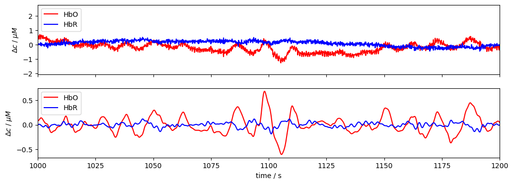
Plot frequency filtered data
Illustrate for a single subject and channel the effect of the bandpass filter.
[5]:
rec = data["sub-01"]
channel = "S5D7"

f, ax = p.subplots(2, 1, figsize=(12, 4), sharex=True)
ax[0].plot(rec["conc"].time, rec["conc"].sel(channel=channel, chromo="HbO"), "r-", label="HbO")
ax[0].plot(rec["conc"].time, rec["conc"].sel(channel=channel, chromo="HbR"), "b-", label="HbR")
ax[1].plot(
    rec["conc_freqfilt"].time,
    rec["conc_freqfilt"].sel(channel=channel, chromo="HbO"),
    "r-",
    label="HbO",
)
ax[1].plot(
    rec["conc_freqfilt"].time,
    rec["conc_freqfilt"].sel(channel=channel, chromo="HbR"),
    "b-",
    label="HbR",
)
ax[0].set_xlim(1000, 1200)
ax[1].set_xlabel("time / s")
ax[0].set_ylabel("$\Delta c$ / $\mu M$")
ax[1].set_ylabel("$\Delta c$ / $\mu M$")
ax[0].legend(loc="upper left")
ax[1].legend(loc="upper left");
[6]:
display(data["sub-01"]["cfepochs"])
<xarray.DataArray 'concentration' (epoch: 60, chromo: 2, channel: 28,
                                   reltime: 196)> Size: 5MB
<Quantity([[[[-1.9479e-02 -1.9950e-02 -2.0945e-02 ... -1.9397e-01 -2.1930e-01
    -2.4552e-01]
   [-1.0442e-02 -1.1375e-02 -1.2845e-02 ... -2.5376e-01 -2.5998e-01
    -2.6454e-01]
   [-1.2500e-02 -8.8897e-03 -5.8428e-03 ... -2.1148e-01 -2.2557e-01
    -2.3975e-01]
   ...
   [ 9.5644e-02  1.0075e-01  1.0499e-01 ... -3.2907e-01 -3.4702e-01
    -3.6405e-01]
   [ 2.0733e-02  2.2404e-02  2.3932e-02 ... -2.9462e-01 -2.9954e-01
    -3.0371e-01]
   [ 1.4324e-03  2.0415e-03  4.1027e-03 ... -3.0974e-01 -3.2710e-01
    -3.4287e-01]]

  [[ 1.4641e-02  6.4301e-03 -1.6853e-03 ... -6.5363e-02 -6.2839e-02
    -5.7220e-02]
   [ 2.0950e-03  5.5313e-03  8.9983e-03 ... -4.8858e-02 -5.4990e-02
    -6.0070e-02]
   [ 4.5053e-02  4.2005e-02  3.9300e-02 ... -4.3936e-02 -4.3039e-02
    -4.0861e-02]
...
   [ 2.8454e-01  2.9324e-01  3.0016e-01 ...  1.0617e-01  1.1339e-01
     1.2119e-01]
   [ 3.4306e-01  3.9592e-01  4.4809e-01 ... -1.8578e-01 -1.7872e-01
    -1.7142e-01]
   [ 6.1801e-01  6.1059e-01  6.0291e-01 ...  1.8868e-01  1.9003e-01
     1.9076e-01]]

  [[ 6.5167e-02  5.7419e-02  4.9134e-02 ...  3.1521e-02  3.2053e-02
     3.1760e-02]
   [ 3.6845e-02  3.4700e-02  3.1450e-02 ... -3.0447e-02 -2.7677e-02
    -2.3868e-02]
   [ 4.8888e-02  3.9980e-02  3.2743e-02 ...  3.0387e-02  3.4824e-02
     3.9630e-02]
   ...
   [ 5.8174e-02  5.3107e-02  4.7739e-02 ... -8.1364e-03 -6.2961e-03
    -5.3040e-03]
   [ 1.5154e-01  1.6202e-01  1.7299e-01 ...  2.6186e-02  3.2992e-02
     3.8859e-02]
   [ 1.5938e-01  1.5348e-01  1.4687e-01 ...  3.8222e-02  4.2833e-02
     4.6774e-02]]]], 'micromolar')>
Coordinates: (3/6)
  * chromo      (chromo) <U3 24B 'HbO' 'HbR'
  * channel     (channel) object 224B 'S1D1' 'S1D2' 'S1D3' ... 'S8D8' 'S8D16'
    ...          ...
    trial_type  (epoch) object 480B 'Tapping/Left' ... 'Tapping/Right'
Dimensions without coordinates: epoch[7]:
all_epochs = xr.concat([rec["cfepochs"] for rec in data.values()], dim="epoch")
all_epochs
[7]:
<xarray.DataArray 'concentration' (epoch: 300, chromo: 2, channel: 28,
                                   reltime: 196)> Size: 26MB
<Quantity([[[[-1.9479e-02 -1.9950e-02 -2.0945e-02 ... -1.9397e-01 -2.1930e-01
    -2.4552e-01]
   [-1.0442e-02 -1.1375e-02 -1.2845e-02 ... -2.5376e-01 -2.5998e-01
    -2.6454e-01]
   [-1.2500e-02 -8.8897e-03 -5.8428e-03 ... -2.1148e-01 -2.2557e-01
    -2.3975e-01]
   ...
   [ 9.5644e-02  1.0075e-01  1.0499e-01 ... -3.2907e-01 -3.4702e-01
    -3.6405e-01]
   [ 2.0733e-02  2.2404e-02  2.3932e-02 ... -2.9462e-01 -2.9954e-01
    -3.0371e-01]
   [ 1.4324e-03  2.0415e-03  4.1027e-03 ... -3.0974e-01 -3.2710e-01
    -3.4287e-01]]

  [[ 1.4641e-02  6.4301e-03 -1.6853e-03 ... -6.5363e-02 -6.2839e-02
    -5.7220e-02]
   [ 2.0950e-03  5.5313e-03  8.9983e-03 ... -4.8858e-02 -5.4990e-02
    -6.0070e-02]
   [ 4.5053e-02  4.2005e-02  3.9300e-02 ... -4.3936e-02 -4.3039e-02
    -4.0861e-02]
...
   [-1.8642e-01 -1.8383e-01 -1.8031e-01 ...  9.3582e-03  1.1076e-02
     1.3423e-02]
   [-2.8335e-01 -2.7513e-01 -2.6600e-01 ... -1.3274e-02 -4.6116e-03
     2.3699e-03]
   [-3.7102e-01 -3.6417e-01 -3.5820e-01 ...  1.8997e-01  1.9610e-01
     2.0283e-01]]

  [[ 6.9413e-02  6.7628e-02  6.5086e-02 ...  2.3354e-02  8.2493e-03
    -6.5091e-03]
   [ 9.3748e-02  7.1599e-02  4.8922e-02 ...  6.0441e-03  3.1716e-02
     4.8579e-02]
   [ 1.3260e-01  1.2931e-01  1.2489e-01 ...  1.8629e-01  1.6657e-01
     1.4594e-01]
   ...
   [ 3.5046e-02  3.1738e-02  2.8594e-02 ...  9.8597e-02  1.0093e-01
     1.0222e-01]
   [ 8.7634e-02  8.3598e-02  8.0126e-02 ...  1.1028e-01  1.0263e-01
     9.5370e-02]
   [-3.3306e-02 -3.6382e-02 -3.7580e-02 ...  4.1337e-03  3.1121e-03
     5.3934e-04]]]], 'micromolar')>
Coordinates: (3/6)
  * chromo      (chromo) <U3 24B 'HbO' 'HbR'
  * channel     (channel) object 224B 'S1D1' 'S1D2' 'S1D3' ... 'S8D8' 'S8D16'
    ...          ...
    trial_type  (epoch) object 2kB 'Tapping/Left' ... 'Tapping/Right'
Dimensions without coordinates: epochBlock Averages
[8]:
# calculate baseline
baseline = all_epochs.sel(reltime=(all_epochs.reltime < 0)).mean("reltime")
# subtract baseline
all_epochs_blcorrected = all_epochs - baseline

# group trials by trial_type. For each group individually average the epoch dimension
blockaverage = all_epochs_blcorrected.groupby("trial_type").mean("epoch")
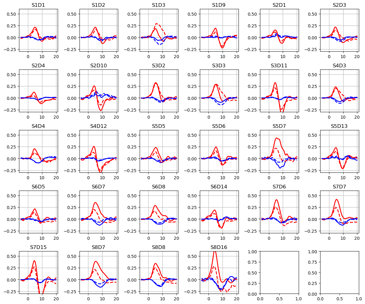
Plotting averaged epochs
[9]:
f, ax = p.subplots(5, 6, figsize=(12, 10))
ax = ax.flatten()
for i_ch, ch in enumerate(blockaverage.channel):
    for ls, trial_type in zip(["-", "--"], blockaverage.trial_type):
        ax[i_ch].plot(
            blockaverage.reltime,
            blockaverage.sel(chromo="HbO", trial_type=trial_type, channel=ch),
            "r",
            lw=2,
            ls=ls,
        )
        ax[i_ch].plot(
            blockaverage.reltime,
            blockaverage.sel(chromo="HbR", trial_type=trial_type, channel=ch),
            "b",
            lw=2,
            ls=ls,
        )
    ax[i_ch].grid(1)
    ax[i_ch].set_title(ch.values)
    ax[i_ch].set_ylim(-0.3, 0.6)

p.tight_layout()
Training a LDA classifier with Scikit-Learn
[10]:
# start with the frequency-filtered, epoched and baseline-corrected concentration data
# discard the samples before the stimulus onset
epochs = all_epochs_blcorrected.sel(reltime=all_epochs_blcorrected.reltime >=0)
# strip units. sklearn would strip them anyway and issue a warning about it.
epochs = epochs.pint.dequantify()

# need to manually tell xarray to create an index for trial_type
epochs = epochs.set_xindex("trial_type")
[11]:
display(epochs)
<xarray.DataArray 'concentration' (epoch: 300, chromo: 2, channel: 28,
                                   reltime: 157)> Size: 21MB
array([[[[-3.6270e-02, -1.8064e-02,  2.0471e-03, ..., -6.8976e-02,
          -9.4304e-02, -1.2053e-01],
         [ 4.6475e-03,  1.1837e-02,  1.9097e-02, ..., -1.5186e-01,
          -1.5808e-01, -1.6264e-01],
         [ 2.4496e-03,  1.2294e-02,  2.3849e-02, ..., -1.3250e-01,
          -1.4658e-01, -1.6077e-01],
         ...,
         [-4.3450e-02, -3.0909e-02, -1.6201e-02, ..., -3.4983e-01,
          -3.6779e-01, -3.8482e-01],
         [ 2.2952e-02,  3.4524e-02,  4.6622e-02, ..., -2.6465e-01,
          -2.6958e-01, -2.7375e-01],
         [-4.2557e-03,  1.3953e-02,  3.3226e-02, ..., -2.5881e-01,
          -2.7617e-01, -2.9194e-01]],

        [[ 1.5914e-02,  1.3944e-02,  1.0925e-02, ..., -7.7108e-02,
          -7.4584e-02, -6.8965e-02],
         [-1.2916e-02, -9.4326e-03, -4.7285e-03, ..., -5.5005e-02,
          -6.1136e-02, -6.6217e-02],
         [-6.1391e-03, -2.1726e-03, -2.9566e-05, ..., -8.1372e-02,
          -8.0476e-02, -7.8297e-02],
...
         [ 1.5353e-01,  1.5630e-01,  1.5688e-01, ...,  6.7293e-02,
           6.9011e-02,  7.1357e-02],
         [ 2.4956e-01,  2.4903e-01,  2.4447e-01, ...,  7.8465e-02,
           8.7128e-02,  9.4109e-02],
         [ 4.8391e-01,  4.8248e-01,  4.7416e-01, ...,  3.1090e-01,
           3.1703e-01,  3.2376e-01]],

        [[-1.5826e-02, -1.2935e-02, -5.2803e-03, ...,  2.3303e-03,
          -1.2774e-02, -2.7533e-02],
         [-1.3622e-02, -1.8221e-02, -2.3395e-02, ...,  1.1320e-02,
           3.6992e-02,  5.3854e-02],
         [-3.5104e-02, -3.3747e-02, -3.9994e-02, ...,  7.3406e-02,
           5.3683e-02,  3.3055e-02],
         ...,
         [ 1.1524e-02,  1.4339e-02,  1.6261e-02, ...,  9.8163e-02,
           1.0049e-01,  1.0178e-01],
         [-5.6057e-02, -5.8393e-02, -5.9799e-02, ...,  6.0866e-02,
           5.3214e-02,  4.5954e-02],
         [ 3.0087e-02,  3.2592e-02,  3.6472e-02, ..., -5.2316e-03,
          -6.2531e-03, -8.8259e-03]]]])
Coordinates: (3/6)
  * chromo      (chromo) <U3 24B 'HbO' 'HbR'
  * channel     (channel) object 224B 'S1D1' 'S1D2' 'S1D3' ... 'S8D8' 'S8D16'
    ...          ...
  * trial_type  (epoch) object 2kB 'Tapping/Left' ... 'Tapping/Right'
Dimensions without coordinates: epoch
Attributes:
units: micromolar[12]:
X = epochs.stack(features=["chromo", "channel", "reltime"])
display(X)
<xarray.DataArray 'concentration' (epoch: 300, features: 8792)> Size: 21MB
array([[-0.0363, -0.0181,  0.002 , ..., -0.0126, -0.0093, -0.0072],
       [ 0.109 ,  0.0983,  0.0847, ..., -0.0343, -0.036 , -0.0378],
       [-0.0203, -0.0267, -0.0325, ..., -0.0187, -0.0155, -0.0115],
       ...,
       [ 0.029 ,  0.0078, -0.0164, ..., -0.0117, -0.0013,  0.0085],
       [-0.2281, -0.2284, -0.2273, ...,  0.0104,  0.0108,  0.0135],
       [ 0.2505,  0.2608,  0.2643, ..., -0.0052, -0.0063, -0.0088]])
Coordinates: (3/7)
    source      (features) object 70kB 'S1' 'S1' 'S1' 'S1' ... 'S8' 'S8' 'S8'
    detector    (features) object 70kB 'D1' 'D1' 'D1' 'D1' ... 'D16' 'D16' 'D16'
    ...          ...
  * reltime     (features) float64 70kB 0.0 0.128 0.256 ... 19.71 19.84 19.97
Dimensions without coordinates: epoch
Attributes:
units: micromolar[13]:
y = xr.apply_ufunc(LabelEncoder().fit_transform, X.trial_type)
display(y)
<xarray.DataArray 'trial_type' (epoch: 300)> Size: 2kB
array([0, 0, 0, 0, 0, 0, 0, 0, 0, 0, 0, 0, 0, 0, 0, 0, 0, 0, 0, 0, 0, 0,
       0, 0, 0, 0, 0, 0, 0, 0, 1, 1, 1, 1, 1, 1, 1, 1, 1, 1, 1, 1, 1, 1,
       1, 1, 1, 1, 1, 1, 1, 1, 1, 1, 1, 1, 1, 1, 1, 1, 0, 0, 0, 0, 0, 0,
       0, 0, 0, 0, 0, 0, 0, 0, 0, 0, 0, 0, 0, 0, 0, 0, 0, 0, 0, 0, 0, 0,
       0, 0, 1, 1, 1, 1, 1, 1, 1, 1, 1, 1, 1, 1, 1, 1, 1, 1, 1, 1, 1, 1,
       1, 1, 1, 1, 1, 1, 1, 1, 1, 1, 0, 0, 0, 0, 0, 0, 0, 0, 0, 0, 0, 0,
       0, 0, 0, 0, 0, 0, 0, 0, 0, 0, 0, 0, 0, 0, 0, 0, 0, 0, 1, 1, 1, 1,
       1, 1, 1, 1, 1, 1, 1, 1, 1, 1, 1, 1, 1, 1, 1, 1, 1, 1, 1, 1, 1, 1,
       1, 1, 1, 1, 0, 0, 0, 0, 0, 0, 0, 0, 0, 0, 0, 0, 0, 0, 0, 0, 0, 0,
       0, 0, 0, 0, 0, 0, 0, 0, 0, 0, 0, 0, 1, 1, 1, 1, 1, 1, 1, 1, 1, 1,
       1, 1, 1, 1, 1, 1, 1, 1, 1, 1, 1, 1, 1, 1, 1, 1, 1, 1, 1, 1, 0, 0,
       0, 0, 0, 0, 0, 0, 0, 0, 0, 0, 0, 0, 0, 0, 0, 0, 0, 0, 0, 0, 0, 0,
       0, 0, 0, 0, 0, 0, 1, 1, 1, 1, 1, 1, 1, 1, 1, 1, 1, 1, 1, 1, 1, 1,
       1, 1, 1, 1, 1, 1, 1, 1, 1, 1, 1, 1, 1, 1])
Coordinates:
  * trial_type  (epoch) object 2kB 'Tapping/Left' ... 'Tapping/Right'
Dimensions without coordinates: epoch[14]:
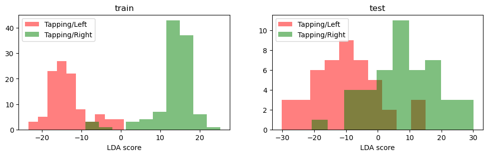
X_train, X_test, y_train, y_test = train_test_split(X, y, test_size=0.3, stratify=y)
classifier = LinearDiscriminantAnalysis(n_components=1).fit(X_train, y_train)
y_pred = classifier.predict(X_test)
print(f"Accuracy: {accuracy_score(y_test, y_pred)}")
Accuracy: 0.8888888888888888
[15]:
f, ax = p.subplots(1, 2, figsize=(12, 3))
for trial_type, c in zip(["Tapping/Left", "Tapping/Right"], ["r", "g"]):
    kw = dict(alpha=0.5, fc=c, label=trial_type)
    ax[0].hist(classifier.decision_function(X_train.sel(trial_type=trial_type)), **kw)
    ax[1].hist(classifier.decision_function(X_test.sel(trial_type=trial_type)), **kw)

ax[0].set_xlabel("LDA score")
ax[1].set_xlabel("LDA score")
ax[0].set_title("train")
ax[1].set_title("test")
ax[0].legend(ncol=1, loc="upper left")
ax[1].legend(ncol=1, loc="upper left");