Image Reconstruction
[1]:
import pyvista as pv
#pv.set_jupyter_backend('html')
pv.set_jupyter_backend('static')
#pv.OFF_SCREEN=True
[2]:
import time

import matplotlib.pyplot as p
import numpy as np
import xarray as xr
from IPython.display import Image

import cedalion
import cedalion.dataclasses as cdc
import cedalion.datasets
import cedalion.geometry.registration
import cedalion.geometry.segmentation
import cedalion.imagereco.forward_model as fw
import cedalion.imagereco.tissue_properties
import cedalion.io
import cedalion.plots
from cedalion.imagereco.solver import pseudo_inverse_stacked

xr.set_options(display_expand_data=False);
Load a finger-tapping dataset
For this demo we load an example finger-tapping recording through cedalion.datasets.get_fingertapping. The file contains a single NIRS element with one block of raw amplitude data.
[3]:
rec = cedalion.datasets.get_fingertapping()
The location of the probes is obtained from the snirf metadata (i.e. /nirs0/probe/)
Note that units (‘m’) are adopted and the coordinate system is named ‘digitized’.
[4]:
geo3d_meas = rec.geo3d
display(geo3d_meas)
<xarray.DataArray (label: 55, digitized: 3)> Size: 1kB
[m] -0.04161 0.0268 0.1299 -0.06477 0.05814 ... 0.06258 0.08226 0.01751 0.06619
Coordinates:
    type     (label) object 440B PointType.SOURCE ... PointType.LANDMARK
  * label    (label) <U3 660B 'S1' 'S2' 'S3' 'S4' 'S5' ... '25' '26' '27' '28'
Dimensions without coordinates: digitized[5]:
cedalion.plots.plot_montage3D(rec["amp"], geo3d_meas)
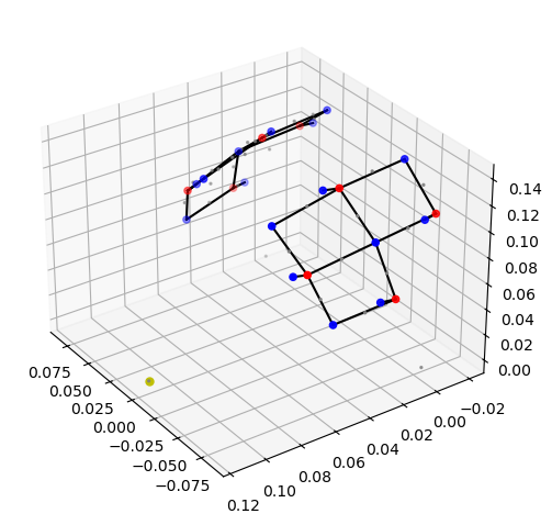
The measurement list is a pandas.DataFrame that describes which source detector pairs form channels.
[6]:
meas_list = rec._measurement_lists["amp"]
display(meas_list.head(5))
| sourceIndex | detectorIndex | wavelengthIndex | wavelengthActual | wavelengthEmissionActual | dataType | dataUnit | dataTypeLabel | dataTypeIndex | sourcePower | detectorGain | moduleIndex | sourceModuleIndex | detectorModuleIndex | channel | source | detector | wavelength | chromo | |
|---|---|---|---|---|---|---|---|---|---|---|---|---|---|---|---|---|---|---|---|
| 0 | 1 | 1 | 1 | None | None | 1 | None | None | 1 | None | None | None | None | None | S1D1 | S1 | D1 | 760.0 | None |
| 1 | 1 | 1 | 2 | None | None | 1 | None | None | 1 | None | None | None | None | None | S1D1 | S1 | D1 | 850.0 | None |
| 2 | 1 | 2 | 1 | None | None | 1 | None | None | 1 | None | None | None | None | None | S1D2 | S1 | D2 | 760.0 | None |
| 3 | 1 | 2 | 2 | None | None | 1 | None | None | 1 | None | None | None | None | None | S1D2 | S1 | D2 | 850.0 | None |
| 4 | 1 | 3 | 1 | None | None | 1 | None | None | 1 | None | None | None | None | None | S1D3 | S1 | D3 | 760.0 | None |
Event/stimulus information is also stored in a pandas.DataFrame. Here events are given more descriptive names:
[7]:
rec.stim.cd.rename_events( {
        "1.0" : "control",
        "2.0" : "Tapping/Left",
        "3.0" : "Tapping/Right"
})
display(rec.stim.groupby("trial_type")[["onset"]].count())
| onset | |
|---|---|
| trial_type | |
| 15.0 | 2 |
| Tapping/Left | 30 |
| Tapping/Right | 30 |
| control | 30 |
(for this demo select 20 seconds after a trial starts at t=117s and transform raw amplitudes to optical density)
Transform CW raw amplitudes to optical density
[8]:
raw_amp = rec["amp"]
rec["od"] = -np.log( raw_amp/ raw_amp.mean("time"))
display(rec["od"])
<xarray.DataArray (channel: 28, wavelength: 2, time: 23239)> Size: 10MB
[] 0.04042 0.0446 0.04422 0.05065 0.04511 ... -0.0113 -0.01109 -0.01094 -0.01317
Coordinates:
  * time        (time) float64 186kB 0.0 0.128 0.256 ... 2.974e+03 2.974e+03
    samples     (time) int64 186kB 0 1 2 3 4 5 ... 23234 23235 23236 23237 23238
  * channel     (channel) object 224B 'S1D1' 'S1D2' 'S1D3' ... 'S8D8' 'S8D16'
    source      (channel) object 224B 'S1' 'S1' 'S1' 'S1' ... 'S8' 'S8' 'S8'
    detector    (channel) object 224B 'D1' 'D2' 'D3' 'D9' ... 'D7' 'D8' 'D16'
* wavelength (wavelength) float64 16B 760.0 850.0Calculate block averages in optical density
[9]:
rec["od_freqfiltered"] = rec["od"].cd.freq_filter(fmin=0.02, fmax=0.5, butter_order=4)
[10]:
epochs = rec["od_freqfiltered"].cd.to_epochs(
rec.stim, # stimulus dataframe
["Tapping/Left", "Tapping/Right"], # select events
before=5, # seconds before stimulus
after=20 # seconds after stimulus
)
# calculate baseline
baseline = epochs.sel(reltime=(epochs.reltime < 0)).mean("reltime")
# subtract baseline
epochs_blcorrected = epochs - baseline
# group trials by trial_type. For each group individually average the epoch dimension
blockaverage = epochs_blcorrected.groupby("trial_type").mean("epoch")
# show results
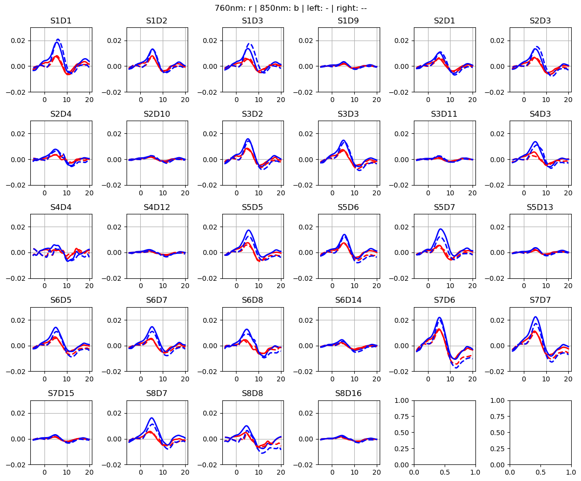
f,ax = p.subplots(5,6, figsize=(12,10))
ax = ax.flatten()
for i_ch, ch in enumerate(blockaverage.channel):
for ls, trial_type in zip(["-", "--"], blockaverage.trial_type):
ax[i_ch].plot(blockaverage.reltime, blockaverage.sel(wavelength=760, trial_type=trial_type, channel=ch), "r", lw=2, ls=ls)
ax[i_ch].plot(blockaverage.reltime, blockaverage.sel(wavelength=850, trial_type=trial_type, channel=ch), "b", lw=2, ls=ls)
ax[i_ch].grid(1)
ax[i_ch].set_title(ch.values)
ax[i_ch].set_ylim(-.02, .03)
p.suptitle("760nm: r | 850nm: b | left: - | right: --")
p.tight_layout()
Load segmented MRI scan
For this example use a segmentation of the Colin27 average brain.
[11]:
SEG_DATADIR, mask_files, landmarks_file = cedalion.datasets.get_colin27_segmentation()
The segmentation masks are in individual niftii files. The dict mask_files maps mask filenames relative to SEG_DATADIR to short labels. These labels describe the tissue type of the mask.
In principle the user is free to choose these labels. However, they are later used to lookup the tissue’s optical properties. So they must be map to one of the tabulated tissue types (c.f. cedalion.imagereco.tissue_properties.TISSUE_LABELS).
The variable landmarks_file holds the path to a file containing landmark positions in scanner space (RAS). This file can be created with Slicer3D.
[12]:
display(SEG_DATADIR)
display(mask_files)
display(landmarks_file)
'/home/runner/.cache/cedalion/colin27_segmentation.zip.unzip/colin27_segmentation'
{'csf': 'mask_csf.nii',
 'gm': 'mask_gray.nii',
 'scalp': 'mask_skin.nii',
 'skull': 'mask_bone.nii',
 'wm': 'mask_white.nii'}
'landmarks.mrk.json'
Coordinate systems
Up to now we have geometrical data from three different coordinate reference systems (CRS):
The optode positions are in one space
CRS='digitized'and the coordinates are in meter. In our example the origin is at the head center and y-axis pointing in the superior direction. Other digitization tools can use other units or coordinate systems.The segmentation masks are in voxel space (
CRS='ijk') in which the voxel edges are aligned with the coordinate axes. Each voxel has unit edge length, i.e. coordinates are dimensionless. Axis-aligned grids are computationally efficient, which is why the photon simulation code (MCX) uses this coordinate system.The voxel space (
CRS='ijk') is related to scanner space (CRS='ras'orCRS='aligned') in which coordinates have physical units and coordinate axes point to the (r)ight, (a)nterior and s(uperior) directions. The relation between both spaces is given through an affine transformation (e.g.t_ijk2ras). When loading the segmentation masks in Slicer3D this transformation is automatically applied. Hence, the picked landmark coordinates are exported in RAS space.The niftii file provides a string label for the scanner space. In this example the RAS space is called ‘aligned’ because the masks are aligned to another MRI scan.
To avoid confusion between these different coordinate systems, cedalion tries to be explicit about which CRS a given point cloud or surface is in.
The TwoSurfaceHeadModel
The photon propagation considers the complete MRI scan, in which each voxel is attributed to one tissue type with its respective optical properties. However, the image reconstruction does not intend to reconstruct absorption changes in each voxel. The inverse problem is simplified, by considering only two surfaces (scalp and brain) and reconstruct only absorption changes in voxels close to these surfaces.
The class cedalion.imagereco.forward_model.TwoSurfaceHeadModel groups together the segmentation mask, landmark positions and affine transformations as well as the scalp and brain surfaces. The brain surface is calculated by grouping together white and gray matter masks. The scalp surface encloses the whole head.
[13]:
head = fw.TwoSurfaceHeadModel.from_segmentation(
    segmentation_dir=SEG_DATADIR,
    mask_files = mask_files,
    landmarks_ras_file=landmarks_file
)
[14]:
head.segmentation_masks
[14]:
<xarray.DataArray (segmentation_type: 5, i: 255, j: 255, k: 189)> Size: 61MB
0 0 0 0 0 0 0 0 0 0 0 0 0 0 0 0 0 0 0 ... 0 0 0 0 0 0 0 0 0 0 0 0 0 0 0 0 0 0 0
Coordinates:
  * segmentation_type  (segmentation_type) <U5 100B 'csf' 'gm' ... 'skull' 'wm'
Dimensions without coordinates: i, j, k
[15]:
head.landmarks
[15]:
<xarray.DataArray (label: 4, ijk: 3)> Size: 96B
[] 127.0 206.8 57.86 128.8 26.05 39.14 55.05 110.9 39.34 202.9 114.0 39.92
Coordinates:
  * label    (label) <U3 48B 'Nz' 'Iz' 'LPA' 'RPA'
    type     (label) object 32B PointType.LANDMARK ... PointType.LANDMARK
Dimensions without coordinates: ijk[16]:
head.brain
[16]:
TrimeshSurface(mesh=<trimesh.Trimesh(vertices.shape=(89995, 3), faces.shape=(180000, 3))>, crs='ijk', units=<Unit('dimensionless')>)
[17]:
head.scalp
[17]:
TrimeshSurface(mesh=<trimesh.Trimesh(vertices.shape=(30242, 3), faces.shape=(60000, 3))>, crs='ijk', units=<Unit('dimensionless')>)
TwoSurfaceHeadModel.from_segmentation converts everything into voxel space (CRS='ijk')
[18]:
head.crs
[18]:
'ijk'
The transformation matrix to translate from voxel to scanner space:
[19]:
head.t_ijk2ras
[19]:
<xarray.DataArray (aligned: 4, ijk: 4)> Size: 128B
[mm] 1.0 0.0 0.0 -127.0 0.0 1.0 0.0 -127.0 0.0 0.0 1.0 -94.0 0.0 0.0 0.0 1.0
Dimensions without coordinates: aligned, ijk
Changing between coordinate systems:
[20]:
head_ras = head.apply_transform(head.t_ijk2ras)
display(head_ras.crs)
display(head_ras.brain)
'aligned'
TrimeshSurface(mesh=<trimesh.Trimesh(vertices.shape=(89995, 3), faces.shape=(180000, 3))>, crs='aligned', units=<Unit('millimeter')>)
Optode Registration
The optode coordinates from the recording must be aligned with the scalp surface. Currently, cedaĺion offers a simple registration method, which finds an affine transformation (scaling, rotating, translating) that matches the landmark positions of the head model and their digitized counter parts. Afterwards, optodes are snapped to the nearest vertex on the scalp.
[21]:
geo3d_snapped_ijk = head.align_and_snap_to_scalp(geo3d_meas)
display(geo3d_snapped_ijk)
<xarray.DataArray (label: 55, ijk: 3)> Size: 1kB
[] 85.61 111.3 166.8 66.62 149.0 129.9 ... 200.3 135.0 99.23 204.1 117.9 100.9
Coordinates:
    type     (label) object 440B PointType.SOURCE ... PointType.LANDMARK
  * label    (label) <U3 660B 'S1' 'S2' 'S3' 'S4' 'S5' ... '25' '26' '27' '28'
Dimensions without coordinates: ijk[22]:
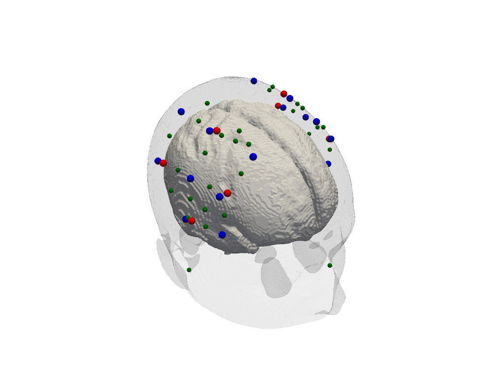
plt = pv.Plotter()
cedalion.plots.plot_surface(plt, head.brain, color="w")
cedalion.plots.plot_surface(plt, head.scalp, opacity=.1)
cedalion.plots.plot_labeled_points(plt, geo3d_snapped_ijk)
plt.show()
Simulate light propagation in tissue
cedalion.imagereco.forward_model.ForwardModel is a wrapper around pmcx. Using the data in the head model it prepares the inputs for either pmcx or NIRFASTer and offers functionality to calculate the sensitivty matrix.
[23]:
fwm = cedalion.imagereco.forward_model.ForwardModel(head, geo3d_snapped_ijk, meas_list)
Run the simulation
The compute_fluence_mcx and compute_fluence_nirfaster methods simulate a light source at each optode position and calculate the fluence in each voxel. By setting RUN_PACKAGE, you can choose between the pmcx or NIRFASTer package to perform this simulation.
[24]:
USE_CACHED = True
RUN_PACKAGE = 'NIRFASTer' # or 'MCX'

if USE_CACHED:
    fluence_all, fluence_at_optodes = cedalion.datasets.get_imagereco_example_fluence()
else:
    if RUN_PACKAGE == 'MCX':
        fluence_all, fluence_at_optodes = fwm.compute_fluence_mcx()
    elif RUN_PACKAGE == 'NIRFASTer':
        fluence_all, fluence_at_optodes = fwm.compute_fluence_nirfaster()
Downloading file 'image_reconstruction_fluence.pickle.gz' from 'https://doc.ml.tu-berlin.de/cedalion/datasets/image_reconstruction_fluence.pickle.gz' to '/home/runner/.cache/cedalion'.
The photon simulation yields the fluence in each voxel for each wavelength.
[25]:
fluence_all
[25]:
<xarray.DataArray (label: 24, wavelength: 2, i: 255, j: 255, k: 189)> Size: 5GB
0.0 0.0 0.0 0.0 0.0 0.0 0.0 0.0 0.0 0.0 ... 0.0 0.0 0.0 0.0 0.0 0.0 0.0 0.0 0.0
Coordinates:
  * label       (label) <U3 288B 'S1' 'S2' 'S3' 'S4' ... 'D13' 'D14' 'D15' 'D16'
    type        (label) object 192B PointType.SOURCE ... PointType.DETECTOR
  * wavelength  (wavelength) float64 16B 760.0 850.0
Dimensions without coordinates: i, j, kAlso, for a each combination of two optodes, the fluence in the voxels at the optode positions is calculated.
[26]:
fluence_at_optodes
[26]:
<xarray.DataArray (optode1: 24, optode2: 24, wavelength: 2)> Size: 9kB
0.06158 0.06158 2.043e-08 2.043e-08 ... 1.492e-08 1.492e-08 0.2147 0.2147
Coordinates:
  * optode1     (optode1) <U3 288B 'S1' 'S2' 'S3' 'S4' ... 'D14' 'D15' 'D16'
  * optode2     (optode2) <U3 288B 'S1' 'S2' 'S3' 'S4' ... 'D14' 'D15' 'D16'
  * wavelength  (wavelength) float64 16B 760.0 850.0
Plot fluence
To illustrate the tissue probed by light travelling from a source to the detector two fluence profiles need to be multiplied.
[27]:
time.sleep(1)

plt = pv.Plotter()

f = fluence_all.loc["S1", 760].values * fluence_all.loc["D1",760].values
f[f<=0] = f[f>0].min()
f = np.log10(f)
vf = pv.wrap(f)

plt.add_volume(
    vf,
    log_scale=False,
    cmap='plasma_r',
    clim=(-10,0),
)
cedalion.plots.plot_surface(plt, head.brain, color="w")
cedalion.plots.plot_labeled_points(plt, geo3d_snapped_ijk)

cog = head.brain.vertices.mean("label").values
plt.camera.position = cog + [-300,30, 150]
plt.camera.focal_point = cog
plt.camera.up = [0,0,1]

plt.show()
/home/runner/micromamba/envs/cedalion/lib/python3.11/site-packages/xarray/core/variable.py:338: UnitStrippedWarning: The unit of the quantity is stripped when downcasting to ndarray.
  data = np.asarray(data)
Calculate the sensitivity matrices
The sensitivity matrix describes the effect of an absorption change at a given surface vertex in the OD recording in a given channel and at given wavelength. The coordinate is_brain holds a mask to distinguish brain and scalp voxels.
[28]:
Adot = fwm.compute_sensitivity(fluence_all, fluence_at_optodes)
Adot
[28]:
<xarray.DataArray (channel: 28, vertex: 120237, wavelength: 2)> Size: 54MB
0.0 0.0 0.0 0.0 2.977e-15 ... 3.159e-20 5.023e-20 5.023e-20 7.523e-19 7.523e-19
Coordinates:
  * channel     (channel) <U5 560B 'S1D1' 'S1D2' 'S1D3' ... 'S8D8' 'S8D16'
  * wavelength  (wavelength) float64 16B 760.0 850.0
    is_brain    (vertex) bool 120kB True True True True ... False False False
Dimensions without coordinates: vertexThe sensitivity Adot has shape (nchannel, nvertex, nwavelenghts). To solve the inverse problem we need a matrix that relates OD in channel space to absorption in image space. Hence, the sensitivity must include the extinction coefficients to translate between OD and concentrations. Furthermore, channels at different wavelengths must be stacked as well vertice and chromophores into new dimensions (flat_channel, flat_vertex):
[29]:
Adot_stacked = fwm.compute_stacked_sensitivity(Adot)
Adot_stacked
/home/runner/micromamba/envs/cedalion/lib/python3.11/site-packages/xarray/core/variable.py:338: UnitStrippedWarning: The unit of the quantity is stripped when downcasting to ndarray.
  data = np.asarray(data)
[29]:
<xarray.DataArray (flat_channel: 56, flat_vertex: 240474)> Size: 108MB
0.0 0.0 4.016e-13 0.0 2.163e-13 ... 2.035e-15 0.0 5.028e-18 7.996e-18 1.198e-16
Dimensions without coordinates: flat_channel, flat_vertex
Invert the sensitivity matrix
[30]:
B = pseudo_inverse_stacked(Adot_stacked)
nvertices = B.shape[0]//2
B = B.assign_coords({"chromo" : ("flat_vertex", ["HbO"]*nvertices  + ["HbR"]* nvertices)})
B = B.set_xindex("chromo")
B
[30]:
<xarray.DataArray (flat_vertex: 240474, flat_channel: 56)> Size: 108MB
0.0 0.0 0.0 0.0 0.0 0.0 ... 1.766e-24 -1.063e-24 -6.122e-24 3.769e-25 3.738e-24
Coordinates:
  * chromo   (flat_vertex) <U3 3MB 'HbO' 'HbO' 'HbO' 'HbO' ... 'HbR' 'HbR' 'HbR'
Dimensions without coordinates: flat_vertex, flat_channel
Calculate concentration changes
the optical density has shape (nchannel, nwavelength, time) -> stack channel and wavelength dimension into new flat_channel dimension
[31]:
blockaverage
[31]:
<xarray.DataArray (trial_type: 2, channel: 28, wavelength: 2, reltime: 196)> Size: 176kB
[] -0.002354 -0.002351 -0.002334 -0.002295 ... -0.0004654 -0.0005121 -0.0005609
Coordinates:
  * channel     (channel) object 224B 'S1D1' 'S1D2' 'S1D3' ... 'S8D8' 'S8D16'
    source      (channel) object 224B 'S1' 'S1' 'S1' 'S1' ... 'S8' 'S8' 'S8'
    detector    (channel) object 224B 'D1' 'D2' 'D3' 'D9' ... 'D7' 'D8' 'D16'
  * wavelength  (wavelength) float64 16B 760.0 850.0
  * reltime     (reltime) float64 2kB -4.992 -4.864 -4.736 ... 19.71 19.84 19.97
* trial_type (trial_type) object 16B 'Tapping/Left' 'Tapping/Right'[32]:
od_stacked = blockaverage.stack({"flat_channel" : ["wavelength", "channel"]})
display(od_stacked)
<xarray.DataArray (trial_type: 2, reltime: 196, flat_channel: 56)> Size: 176kB
[] -0.002354 -0.001524 -0.001609 -0.0005054 ... -0.002499 -0.008621 -0.0005609
Coordinates:
    source        (flat_channel) object 448B 'S1' 'S1' 'S1' ... 'S8' 'S8' 'S8'
    detector      (flat_channel) object 448B 'D1' 'D2' 'D3' ... 'D7' 'D8' 'D16'
  * reltime       (reltime) float64 2kB -4.992 -4.864 -4.736 ... 19.84 19.97
  * trial_type    (trial_type) object 16B 'Tapping/Left' 'Tapping/Right'
  * flat_channel  (flat_channel) object 448B MultiIndex
  * wavelength    (flat_channel) float64 448B 760.0 760.0 760.0 ... 850.0 850.0
* channel (flat_channel) object 448B 'S1D1' 'S1D2' ... 'S8D8' 'S8D16'multiply with the inverted sensitivity matrix. contracts over flat_channel and the flat_vertex dimension remains
[33]:
dC = B @ od_stacked
dC
[33]:
<xarray.DataArray (flat_vertex: 240474, trial_type: 2, reltime: 196)> Size: 754MB
[] 0.0 0.0 0.0 0.0 0.0 ... -9.449e-27 -8.761e-27 -8.353e-27 -8.166e-27 -8.13e-27
Coordinates:
  * chromo      (flat_vertex) <U3 3MB 'HbO' 'HbO' 'HbO' ... 'HbR' 'HbR' 'HbR'
  * reltime     (reltime) float64 2kB -4.992 -4.864 -4.736 ... 19.71 19.84 19.97
  * trial_type  (trial_type) object 16B 'Tapping/Left' 'Tapping/Right'
Dimensions without coordinates: flat_vertex
Plot concentration changes
Using functionality from pyvista and VTK plot the concentration changes on the brain surface
[34]:
b = cdc.VTKSurface.from_trimeshsurface(head.brain)
b = pv.wrap(b.mesh)
[35]:
# plot brain surface

for trial_type, gif_fname in [("Tapping/Left", "hbo_left.gif"), ("Tapping/Right", "hbo_right.gif")]:

    hbo = dC.sel(chromo="HbO", trial_type=trial_type).pint.dequantify() / 1e-6 # FIXME unit handling
    hbo_brain = hbo[(Adot.is_brain == True).values,:]

    ntimes = hbo.sizes["reltime"]

    b = cdc.VTKSurface.from_trimeshsurface(head.brain)
    b = pv.wrap(b.mesh)
    b["reco_hbo"] = (hbo_brain[:,0] - hbo_brain[:,0])

    plt = pv.Plotter()

    plt.add_mesh(
        b,
        scalars="reco_hbo",
        cmap='seismic', # 'gist_earth_r',
        clim=(-0.3,0.3),
        scalar_bar_args = {"title" : "HbO / µM"}
    )

    cedalion.plots.plot_labeled_points(plt, geo3d_snapped_ijk)


    tl = lambda tt : f"{trial_type} HbO rel. time: {tt:.3f} s"
    time_label = plt.add_text(tl(0))

    cog = head.brain.vertices.mean("label").values
    plt.camera.position = cog + [0,0,400]
    plt.camera.focal_point = cog
    plt.camera.up = [0,1,0]
    plt.reset_camera()

    plt.open_gif(gif_fname)

    for i in range(0,ntimes,3):
        b["reco_hbo"] = (hbo_brain[:,i] - hbo_brain[:,0])
        time_label.set_text("upper_left", tl(hbo_brain.reltime[i]))

        plt.write_frame()

    plt.close()
/home/runner/micromamba/envs/cedalion/lib/python3.11/site-packages/xarray/core/variable.py:338: UnitStrippedWarning: The unit of the quantity is stripped when downcasting to ndarray.
  data = np.asarray(data)
/home/runner/micromamba/envs/cedalion/lib/python3.11/site-packages/xarray/core/variable.py:338: UnitStrippedWarning: The unit of the quantity is stripped when downcasting to ndarray.
  data = np.asarray(data)
[36]:
display(Image(data=open("hbo_left.gif",'rb').read(), format='png'))
display(Image(data=open("hbo_right.gif",'rb').read(), format='png'))