Photogrammetric Optode Coregistration

[1]:

import logging
logging.basicConfig()
logging.getLogger("cedalion").setLevel(logging.DEBUG)

import cedalion.io
import cedalion.plots
from cedalion.geometry.photogrammetry.processors import ColoredStickerProcessor
from cedalion.datasets import get_photogrammetry_example_scan
import xarray as xr
import pyvista as pv

xr.set_options(display_expand_data=False);

INFO:pysnirf2:Library loaded by process 3130

Choose between interactive and static 3D plots

[2]:

pv.set_jupyter_backend("static")  # uncomment for static rendering
#pv.set_jupyter_backend("client")  # uncomment for interactive rendering
#pv.set_jupyter_backend("html")

Use cedalion.io.read_einstar_obj to read the textured triangle mesh produced by the Einstar scanner.

[3]:

example_scan_fname = get_photogrammetry_example_scan()
s = cedalion.io.read_einstar_obj(example_scan_fname)

Downloading file 'photogrammetry_example_scan.zip' from 'https://doc.ml.tu-berlin.de/cedalion/datasets/photogrammetry_example_scan.zip' to '/home/runner/.cache/cedalion'.
Unzipping contents of '/home/runner/.cache/cedalion/photogrammetry_example_scan.zip' to '/home/runner/.cache/cedalion/photogrammetry_example_scan.zip.unzip'

Processors are meant to analyze the textured mesh and extract positions. The ColoredStickerProcessor searches for colored circular areas. The colors must be specified by their ranges in hue and value. These can for example be found by usig a color pipette tool on the texture file.

In the following to classes of stickers are searched: “O(ptodes)” in blue and “L(andmarks” in yellow.

[4]:

processor = ColoredStickerProcessor(
    colors={
        "O" : ((0.11, 0.21, 0.8, 1)), # (hue_min, hue_max, value_min, value_max)
        "L" : ((0.25, 0.37, 0.35, 0.6))
    }
)

[5]:

sticker_centers, normals, details = processor.process(s, details=True)

DEBUG:cedalion:skipping non-circuluar cluster 37

[6]:

display(sticker_centers)

<xarray.DataArray (label: 67, digitized: 3)> Size: 2kB
[mm] 95.06 4.429 646.8 77.58 -1.072 408.8 ... -60.75 562.5 82.59 80.29 498.7
Coordinates:
  * label    (label) <U4 1kB 'O-01' 'O-02' 'O-03' ... 'L-04' 'L-05' 'L-06'
    type     (label) object 536B PointType.UNKNOWN ... PointType.UNKNOWN
    group    (label) <U1 268B 'O' 'O' 'O' 'O' 'O' 'O' ... 'L' 'L' 'L' 'L' 'L'
Dimensions without coordinates: digitized

Visualize the surface and extraced results.

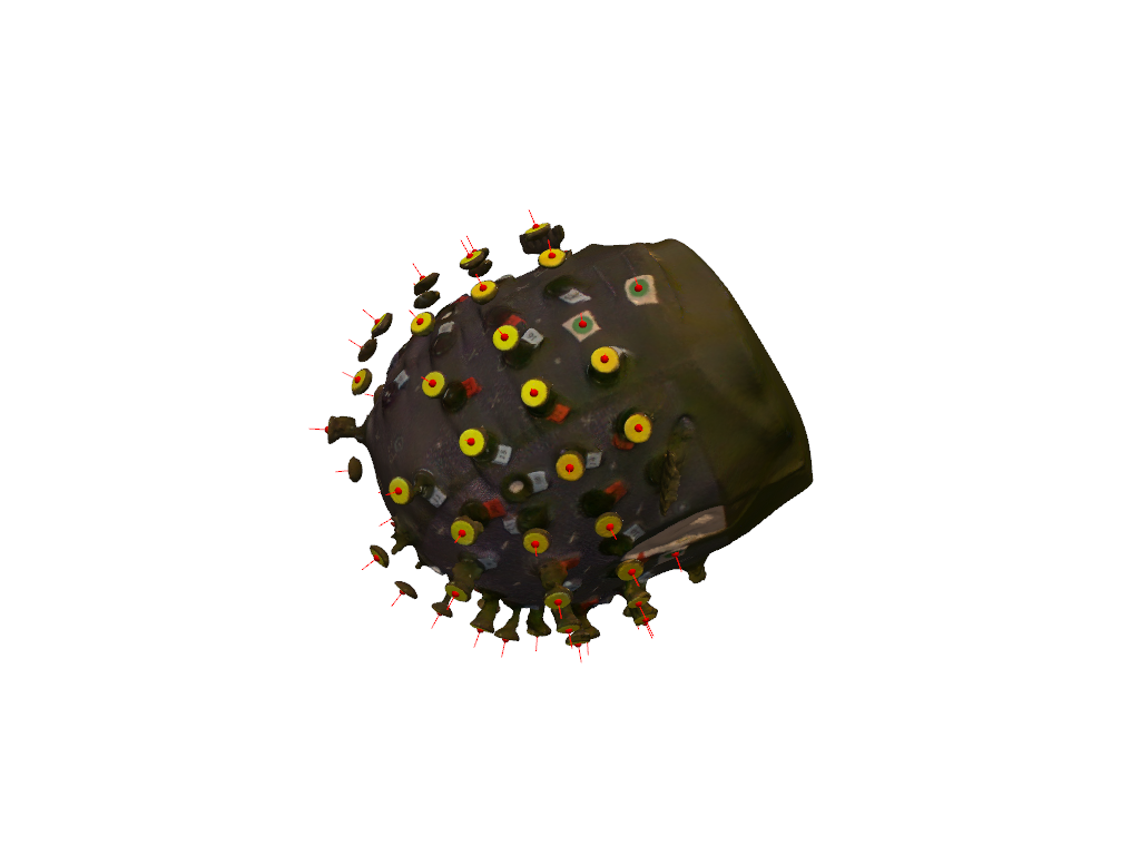
[7]:

plt = pv.Plotter()
cedalion.plots.plot_surface(plt, s, opacity=1.0)
cedalion.plots.plot_labeled_points(plt, sticker_centers, color="r")
cedalion.plots.plot_vector_field(plt, sticker_centers, normals)
plt.show()

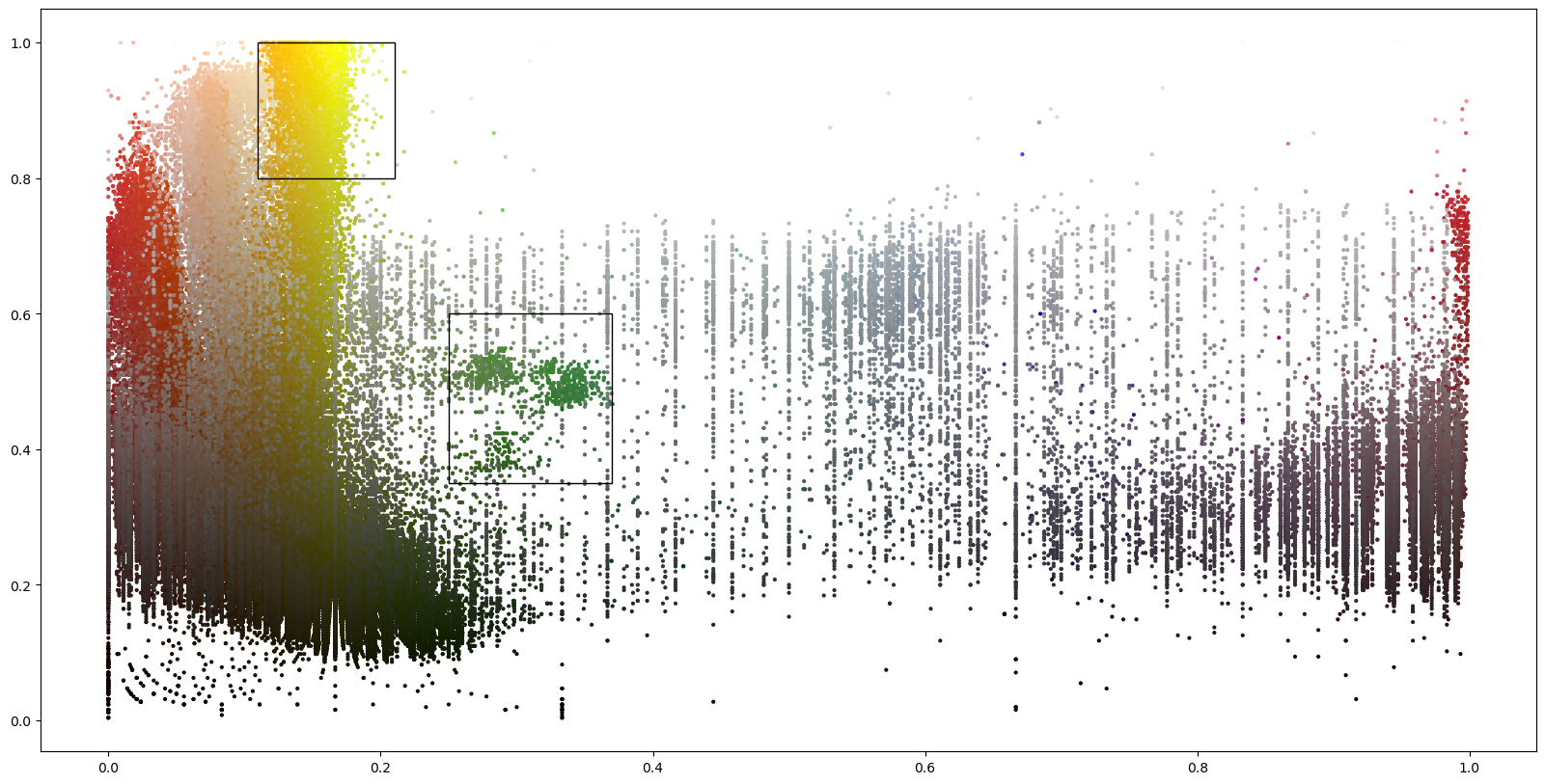
../_images/examples_photogrammetry_11_0.png

The details object is meant as a container for debuging information. It also provides plotting functionality.The following scatter plot shows the vertex colors in the hue-value plane in which the vertex classification operates.

[8]:

details.plot_vertex_colors()

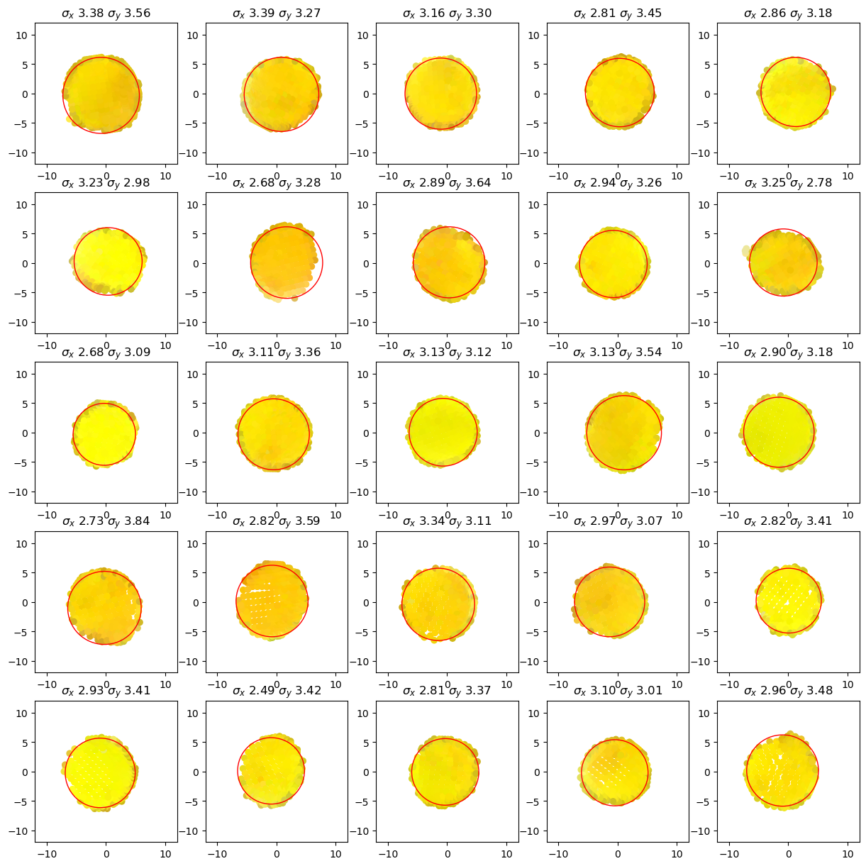
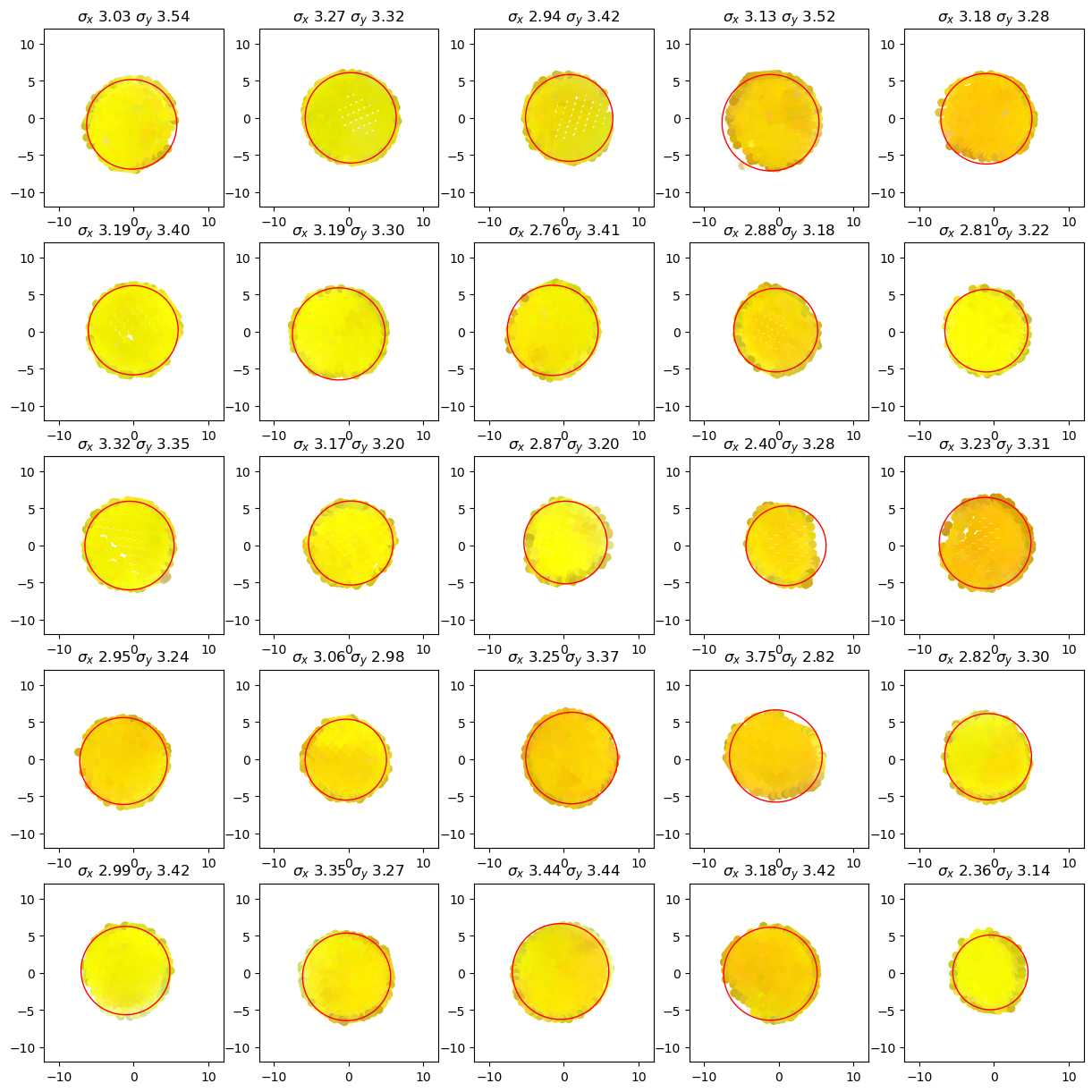
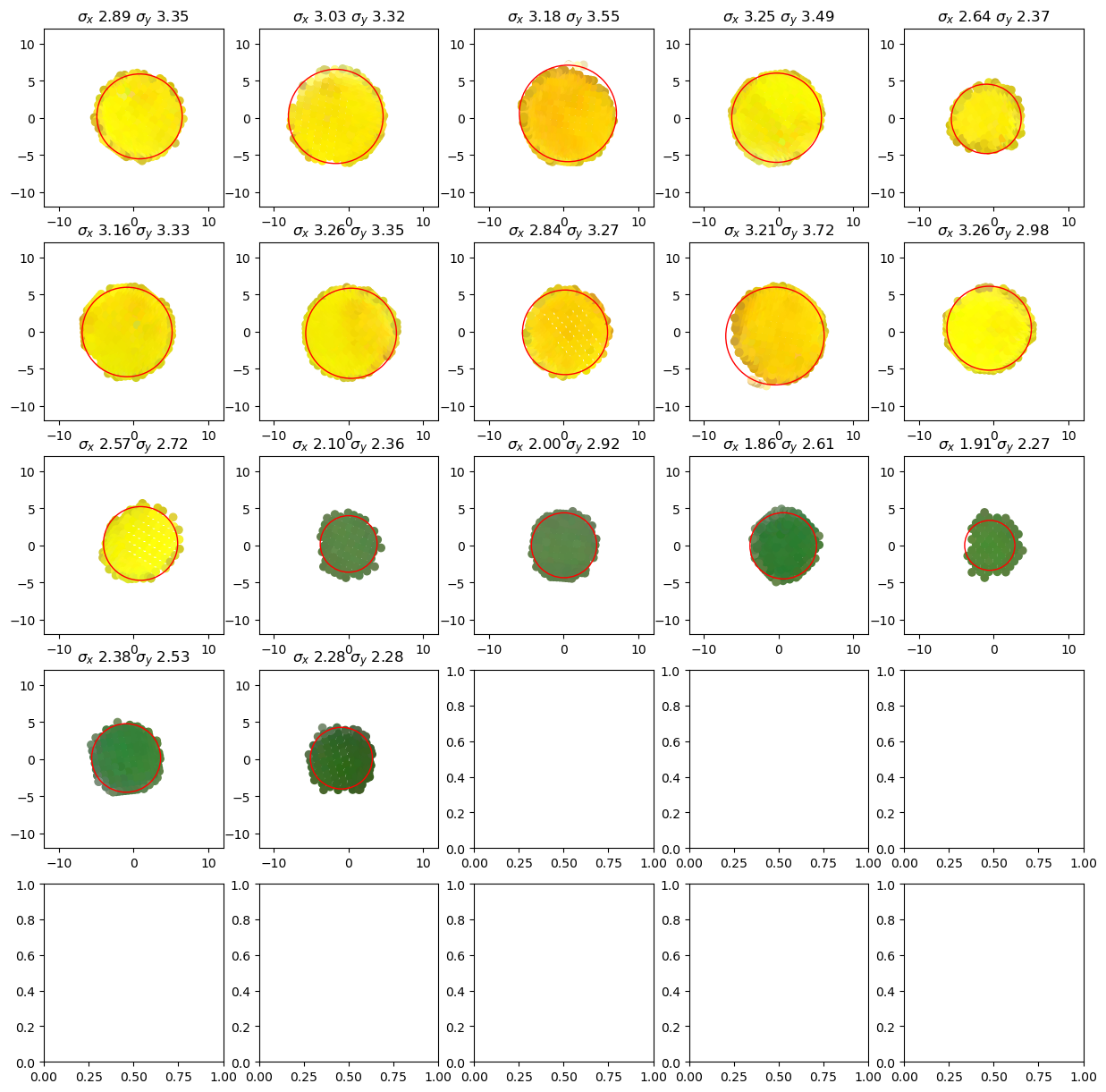
../_images/examples_photogrammetry_13_0.png

The following plots show for each cluster (tentative group of sticker vertices) The vertex positions perpendicular to the sticker normal as well as the minimum enclosing circle which is used to find the sticker’s center.

[9]:

details.plot_cluster_circles()

../_images/examples_photogrammetry_15_0.png

../_images/examples_photogrammetry_15_1.png

../_images/examples_photogrammetry_15_2.png

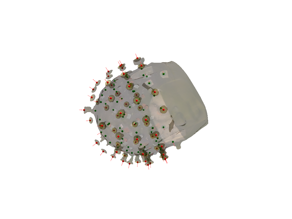
Finally, to get from the sticker centers to the scalp coordinates we have to subtract the lenght of the optodes in the direction of the normals:

[10]:

optode_length = 22.6 * cedalion.units.mm

scalp_coords = sticker_centers.copy()
mask_optodes = sticker_centers.group == 'O'
scalp_coords[mask_optodes] = sticker_centers[mask_optodes] - optode_length*normals[mask_optodes]

[11]:

display(scalp_coords)

<xarray.DataArray (label: 67, digitized: 3)> Size: 2kB
[mm] 90.52 5.402 624.7 77.72 -4.772 431.1 ... -60.75 562.5 82.59 80.29 498.7
Coordinates:
  * label    (label) <U4 1kB 'O-01' 'O-02' 'O-03' ... 'L-04' 'L-05' 'L-06'
    type     (label) object 536B PointType.UNKNOWN ... PointType.UNKNOWN
    group    (label) <U1 268B 'O' 'O' 'O' 'O' 'O' 'O' ... 'L' 'L' 'L' 'L' 'L'
Dimensions without coordinates: digitized

[12]:

plt = pv.Plotter()
cedalion.plots.plot_surface(plt, s, opacity=0.3)
cedalion.plots.plot_labeled_points(plt, sticker_centers, color="r")
cedalion.plots.plot_labeled_points(plt, scalp_coords, color="g")
cedalion.plots.plot_vector_field(plt, sticker_centers, normals)
plt.show()

../_images/examples_photogrammetry_19_0.png

TBD: The found landmark and optode positions must still be matched to a montage in order to distinguish between sources and detectors and to assign the correct labels.